Integrated Modeling of Tokamak Plasmas

The stability analysis of the KSTAR discharge 7328 is presented below. The initial settings for this study are based on the pedestal parameters and other plasma parameters that are outlined in the case s17.

The ballooning stability boundary is shown on this plot. The peeling stability boundary is also identified. However, the parallel current density that will make the peeling modes unstable are significantly large and are in the range of . The and toroidal mode numbers that are close to the experimentally observed modes are marked on the diagram. Note, the transition from to will be associated with very small changes in the normalized plasma density and with relatively large changes in the parallel current density. The pedestal plasma density for both equilibria was , the pedestal temperatures were and for the cases of and unstable modes correspondingly. The bootstrap current was computed using the Sauter formula for the case of mode and using the Sauter formula with the scaling factor of 1.2 for the case of mode.

If the values of the plasma temperatures is on the upper boundary of the experimental error bar (or slightly above the error bar), the likely conclusion is that the Sauter formula for KSTAR pedestal parameters under-predicts the bootstrap current.

The XGC0 code has been also used to model the radial electric field and poloidal velocity profiles for the KSTAR discharge 7328. The profiles for the three cases with different collisionalities that are described in the previous post are shown below.

Radial electric field (outside midplane)

Poloidal velocity profiles

The poloidal velocity and radial electric field in the H-mode pedestal region strongly depend on the plasma collisionality.

NIMROD and BOUT++ results are compared for the case gs11-t00-t073 that is generated using the procedure described in the previous post. The growth rates computed using the NIMROD and BOUT++ codes are compared below.

The NIMROD results and BOUT++ results that are shown as blue curve are run with . However, the constant resistivity profile is used in these simulations. There are several conclusions from these and other NIMROD/BOUT++ comparison simulations:

1. The resistivity profiles and a proper account for the diamagnetic effects are important;
2. The parallel viscosity effects have relatively weak effect on the ELM dynamics at least during a linear stage of a crash.

The following steps are used for KSTAR equilibrium reconstruction:

1. Generate a new inverse equilibrium using the TOQ equilibrium solver. There are certain assumptions for the plasma profiles in the process. In particular, the case s13-t00-06 uses these parameters for the plasma profiles:

    modelp=27
    nedge13=0.7
    nped13=2.6
    ncore13=4.6
    nexpin=1.1
    nexpout=1.1
    tedgeEV=70.
    tpedEV= 500
    tcoreEV=2600.0
    texpin=1.1
    texpout=2. 
    widthp=.07
    xphalf=.91

2. The DCON stability code is used the test the stability of resulting equilibrium
3. The plasma profiles from TOQ are interpolated to the TEQ grid in Corsica. These profile include the plasma pressure and safefy factor.
4. The interpolated plasma pressure and the interpolated safety factor are sent to TEQ to generated new geqdsk files that would include the vacuum field solution.
   The Corsica psave and qsave variables are used.
   • We start with the original sav-file for this discharge: 

     caltrans 007328_4400.sav  -probname ss-test kstar.bas

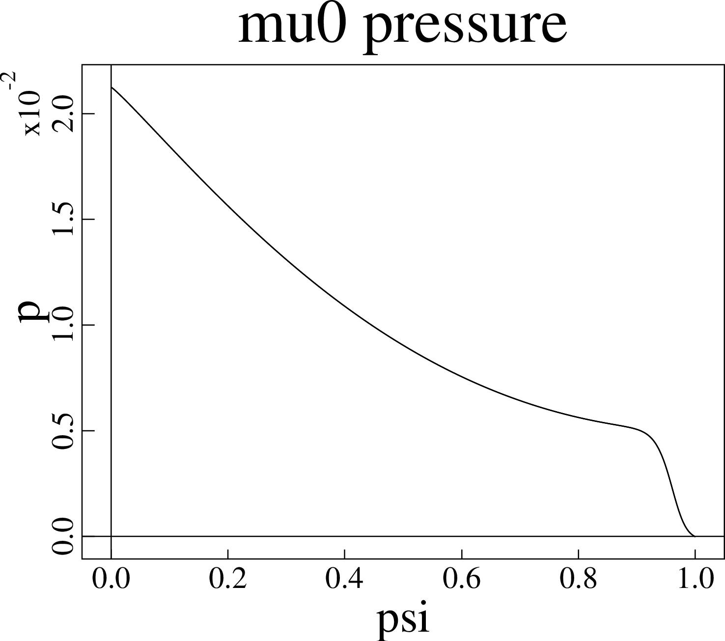
   • Then, we update the pressure profile and generate new inverse solution:

     thetac=1e-3; epsrk=5.e-9; nht=5000; start_inv
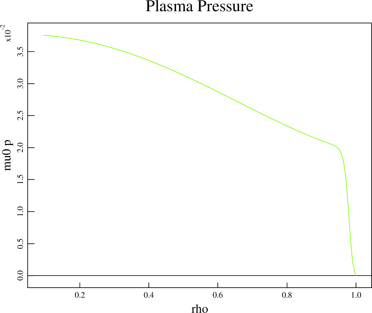
     psave( 1: 26)=[4.0652e+05,4.0636e+05,4.0589e+05,4.0510e+05,4.0400e+05,4.0259e+05,4.0085e+05,3.9876e+05,3.9636e+05,3.9354e+05,3.9038e+05,3.8681e+05,3.8290e+05,3.7861e+05,3.7397e+05,3.6897e+05,3.6364e+05,3.5798e+05,3.5201e+05,3.4573e+05,3.3917e+05,3.3235e+05,3.2528e+05,3.1798e+05,3.1047e+05,3.0278e+05]
     psave( 27: 52)=[2.9493e+05,2.8693e+05,2.7881e+05,2.7061e+05,2.6233e+05,2.5400e+05,2.4565e+05,2.3729e+05,2.2897e+05,2.2067e+05,2.1246e+05,2.0432e+05,1.9630e+05,1.8841e+05,1.8065e+05,1.7307e+05,1.6566e+05,1.5845e+05,1.5144e+05,1.4466e+05,1.3810e+05,1.3179e+05,1.2572e+05,1.1991e+05,1.1436e+05,1.0907e+05]
     psave( 53: 78)=[1.0405e+05,9.9302e+04,9.4818e+04,9.0599e+04,8.6643e+04,8.2945e+04,7.9499e+04,7.6298e+04,7.3334e+04,7.0596e+04,6.8068e+04,6.5736e+04,6.3577e+04,6.1565e+04,5.9667e+04,5.7842e+04,5.6037e+04,5.4183e+04,5.2207e+04,5.0025e+04,4.7558e+04,4.4737e+04,4.1586e+04,3.8103e+04,3.4179e+04,2.9900e+04]
     psave( 79:101)=[2.5535e+04,2.1282e+04,1.7332e+04,1.3874e+04,1.0920e+04,8.4769e+03,6.5566e+03,5.0422e+03,3.8616e+03,2.9488e+03,2.2444e+03,1.6993e+03,1.2741e+03,9.5421e+02,7.0459e+02,5.0154e+02,3.5481e+02,2.3120e+02,1.4798e+02,8.3140e+01,3.6807e+01,8.9772e+00,3.4489e+00]
     teq_inv(0,1); teq_inv(0,1)

     The inverse equilibrium solver is called with the options to keep the plasma current unaltered. We run the solver two times, because the solver has a tendency to inverse the plasma current in the equilibrium solution.

   • Then, the direct solution is generated using direct TEQ solver:

     inv_eq=0; inv_k=0; run

   • The solution is stored in a new sav-file

     saveq("s13-t00-01.sav")

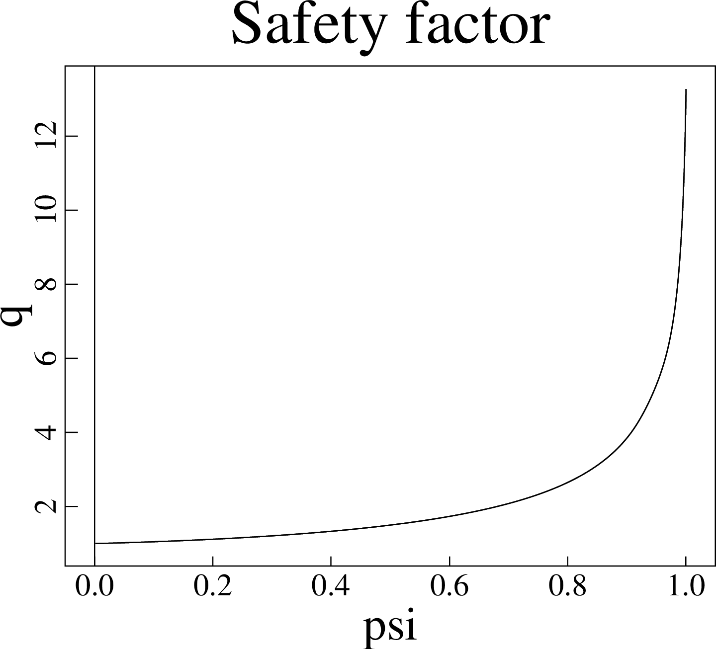
   • The q-prifiles are being updated now:

     thetac=1e-3; epsrk=5.e-9; nht=5000; start_inv

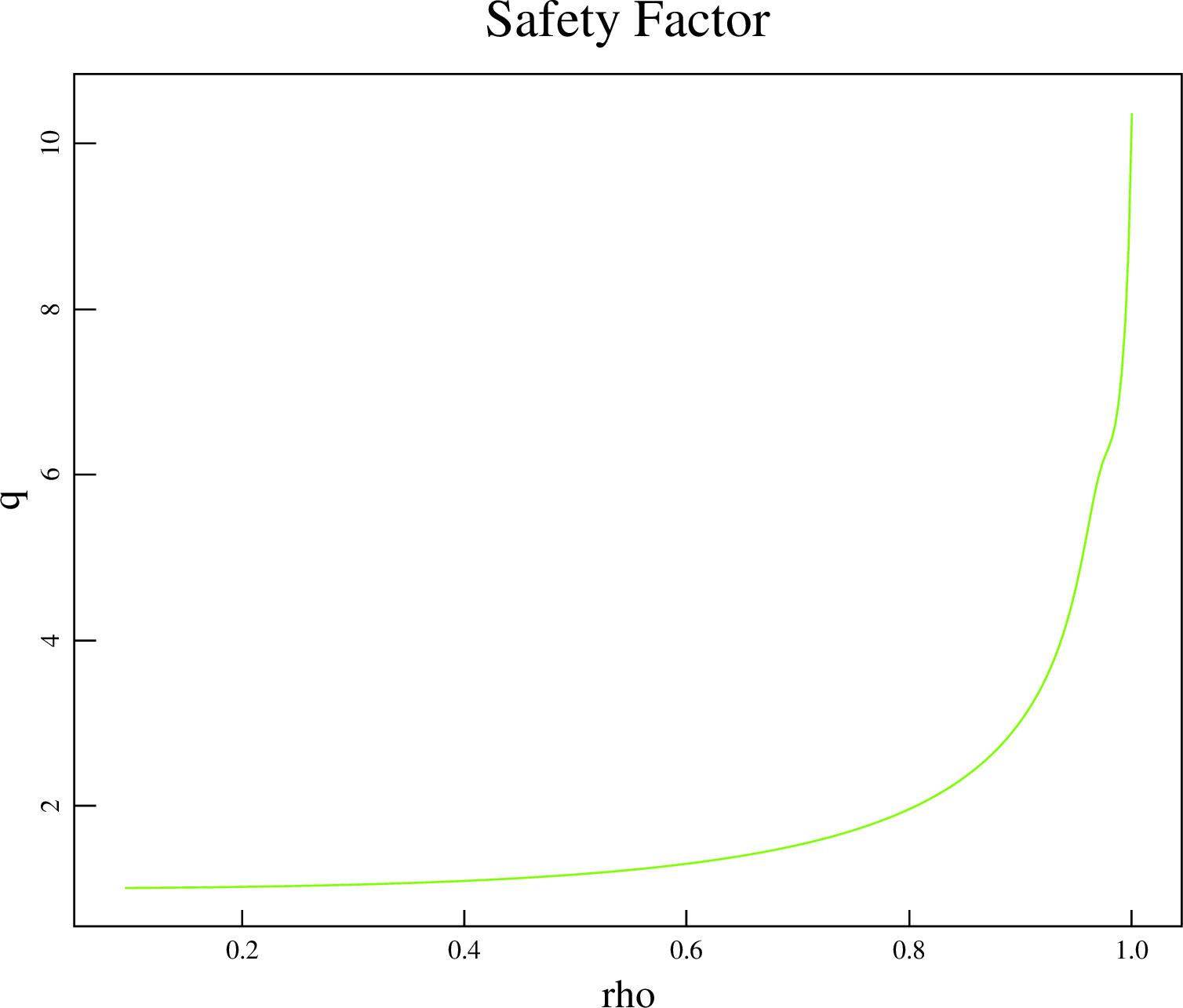
     qsave( 1: 26)=[1.3999e+00,1.4000e+00,1.4006e+00,1.4014e+00,1.4026e+00,1.4041e+00,1.4060e+00,1.4082e+00,1.4108e+00,1.4137e+00,1.4170e+00,1.4207e+00,1.4248e+00,1.4292e+00,1.4341e+00,1.4394e+00,1.4451e+00,1.4513e+00,1.4579e+00,1.4650e+00,1.4726e+00,1.4806e+00,1.4892e+00,1.4983e+00,1.5079e+00,1.5181e+00]
     qsave( 27: 52)=[1.5289e+00,1.5403e+00,1.5524e+00,1.5650e+00,1.5784e+00,1.5924e+00,1.6072e+00,1.6227e+00,1.6390e+00,1.6560e+00,1.6740e+00,1.6927e+00,1.7124e+00,1.7331e+00,1.7546e+00,1.7773e+00,1.8009e+00,1.8257e+00,1.8515e+00,1.8786e+00,1.9070e+00,1.9366e+00,1.9675e+00,1.9998e+00,2.0336e+00,2.0689e+00]
     qsave( 53: 78)=[2.1059e+00,2.1445e+00,2.1848e+00,2.2270e+00,2.2711e+00,2.3171e+00,2.3653e+00,2.4157e+00,2.4684e+00,2.5236e+00,2.5813e+00,2.6418e+00,2.7051e+00,2.7715e+00,2.8411e+00,2.9142e+00,2.9910e+00,3.0719e+00,3.1572e+00,3.2472e+00,3.3424e+00,3.4432e+00,3.5509e+00,3.6655e+00,3.7876e+00,3.9196e+00]
     qsave( 79:101)=[4.0602e+00,4.2122e+00,4.3736e+00,4.5492e+00,4.7362e+00,4.9360e+00,5.1541e+00,5.3890e+00,5.6429e+00,5.9183e+00,6.2180e+00,6.5436e+00,6.8934e+00,7.2872e+00,7.7253e+00,8.1641e+00,8.6979e+00,9.1615e+00,9.8188e+00,1.0331e+01,1.0697e+01,1.0917e+01,1.0960e+01]
     teq_inv(0,1); teq_inv(0,1)

   • New direct solution is generated again. The solution will include the update plasma pressure and q profiles:

     inv_eq=0; inv_k=0; run

     saveq("s13-t00-02.sav")

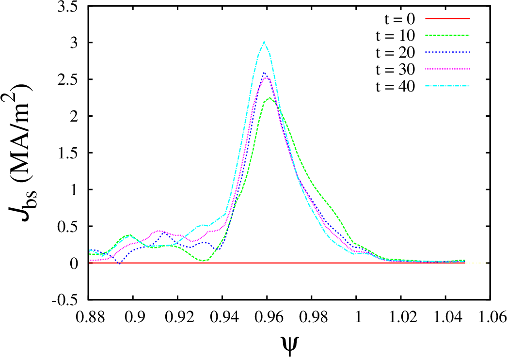
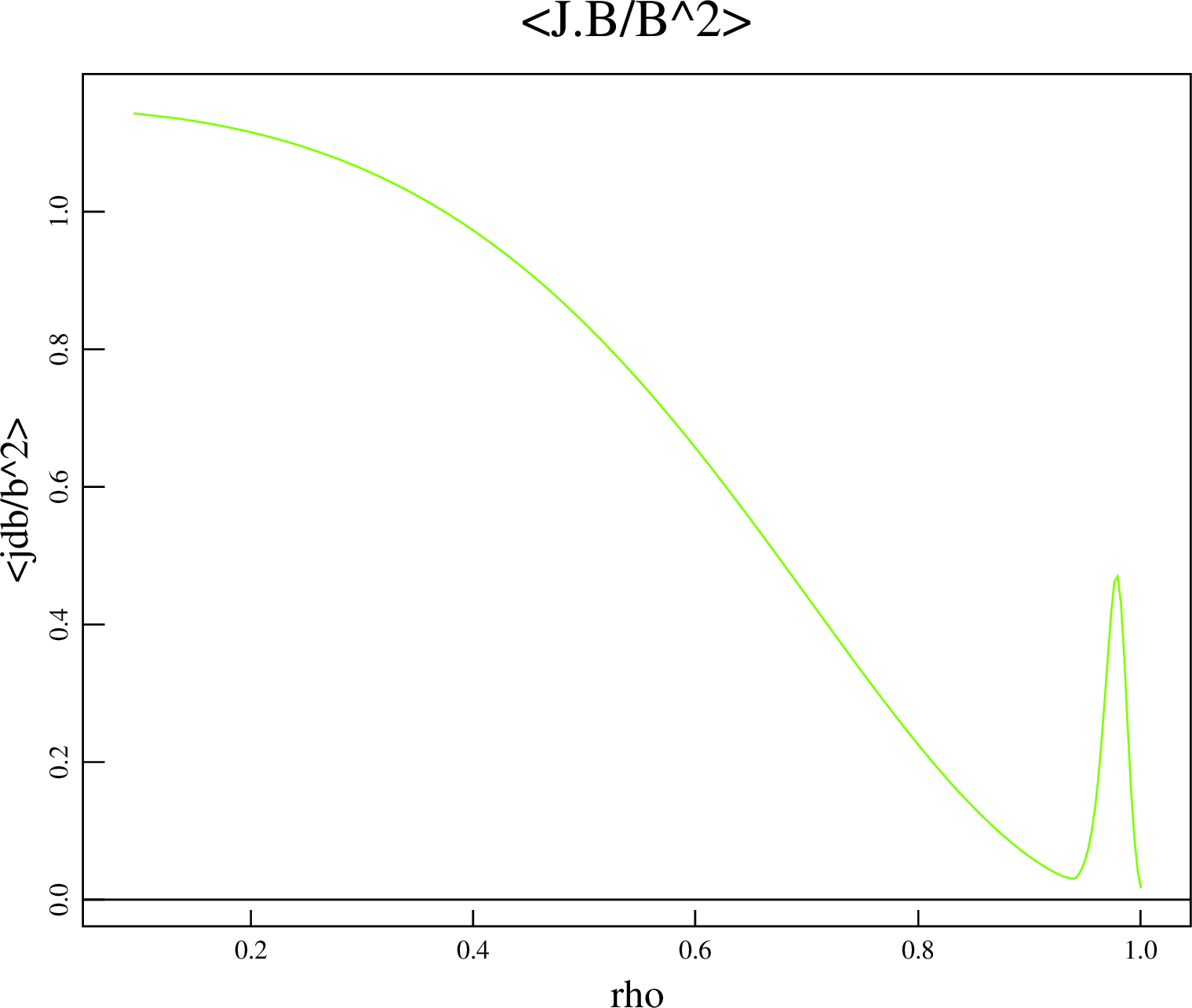
   • Now, we need to ensure that the bootstrap current is properly included. In order to do this, we will exclude the edge current from the jparsrf and will replace it with the bootstrap current from the Sauter model:

     jparsave(81:101)=jparsave(80)

     real ndens=psibar; ndens=2.6e19
     real prbs=psave/10./2.
     real tebs=prbs/ndens/1.602e-19
     real zeffbs=psave; zeffbs=1.
     real pbeambs=psibar; pbeambs=0.
     read jbootstrap.bas

     real jbs1 = jbootstrap(prbs,ndens,tebs,tebs,zeffbs, pbeambs, 1., 1., 0.)
     real jbs0 = jbs1(:,1)
     real foo1=tanh((1.01-psibar)/0.05)
     real foo2=(1+tanh((psibar-0.7)/0.05))/2.
     jparsave=jparsave*foo1+jbs0/bsqrf*foo2

   • Run a sequence of inverse and direct equilibrium solvers ensuring the the plasma current does not change:

     thetac=1e-3; residj=1e-9; nht=5000; start_inv
     jparsave=jparsave*foo1+jbs0/bsqrf*foo2
     nf; plot [jparsrf,jparsave], asrf+rsrf
     teq_inv(3,0); teq_inv(0,1); teq_inv(0,1)
     inv_eq=0; inv_k=0; run
     saveq("s13-t00-03.sav")

   • Increase the resolution in the direct equilibrium solution to 257×257 (at least):

     gridup; run; saveq("s13-t00-04.sav")

     gridup; run; saveq("s13-t00-05.sav")

   • Save the new geqdsk file

     weqdsk

   • Note, the the resolution for the inverse solver is also important and it might be useful to increase it by changing the values of map and msrf (theta and psi dimensions in the inverse solve) and running the inverse solver.
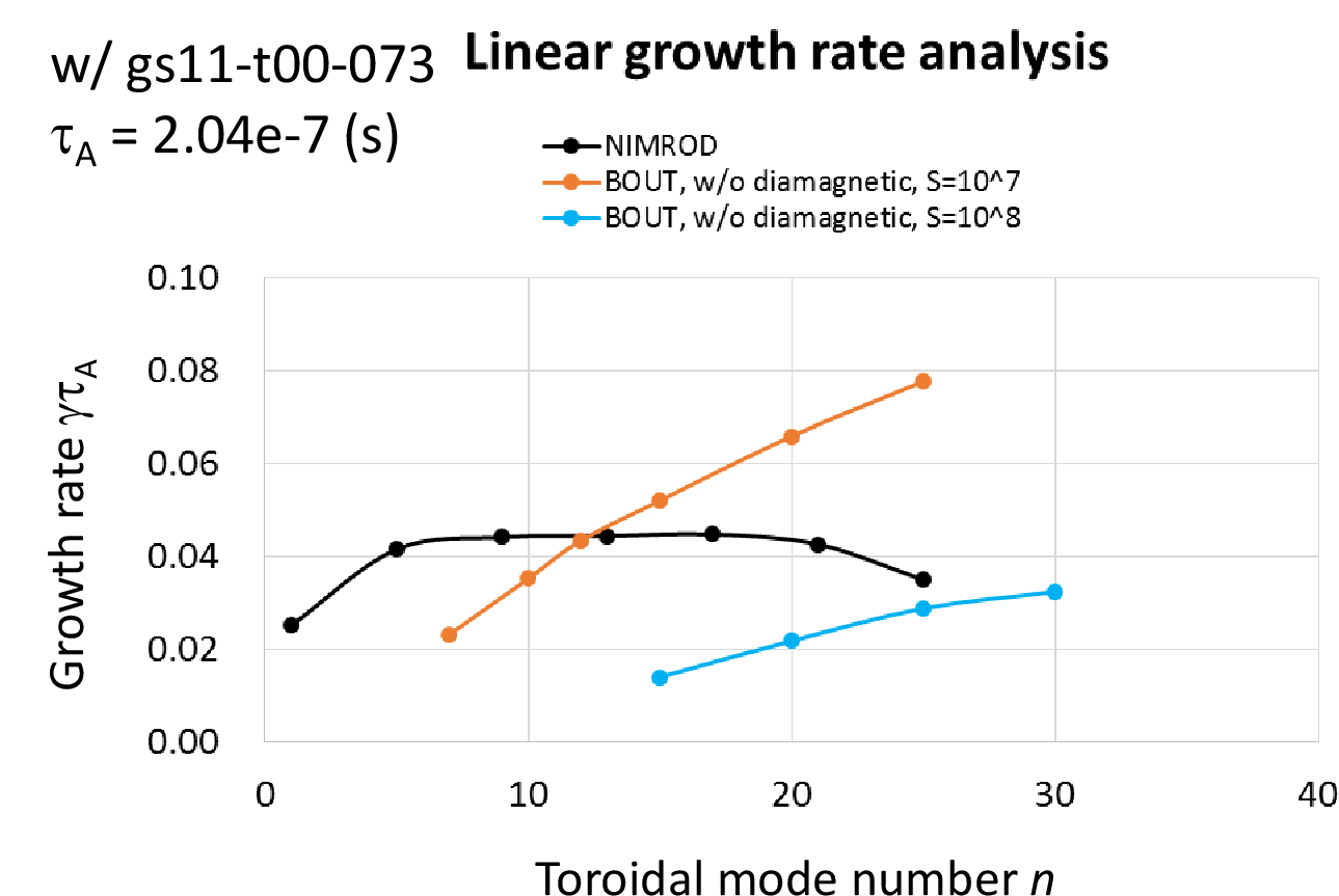
5. The new geqdsk can be used in the MHD stability codes or with extended MHD codes for further analysis. In order to modify this equilibrium even further, one can modify the pressure profile and parallel current density profile using the last sav-file. An example  below shows how to change the slope in the H-mode pedestal without changing the pedestal width:

    thetac=1e-3; epsrk=5.e-9; nht=5000; start_inv
    real foo2=(1+tanh((psibar-0.90)/0.02))/2.
    real foo1=(1-tanh((psibar-0.91)/0.02))/2.
    psave=prsrf*(2-(foo1+foo2))
    teq_inv(0,1); teq_inv(0,1)
    inv_eq=0; inv_k=0; run
    saveq("s13-t01-01.sav"); weqdsk

   Changes in the plasma pressure are shown below:
   

6. The final layout looks as shown:
   

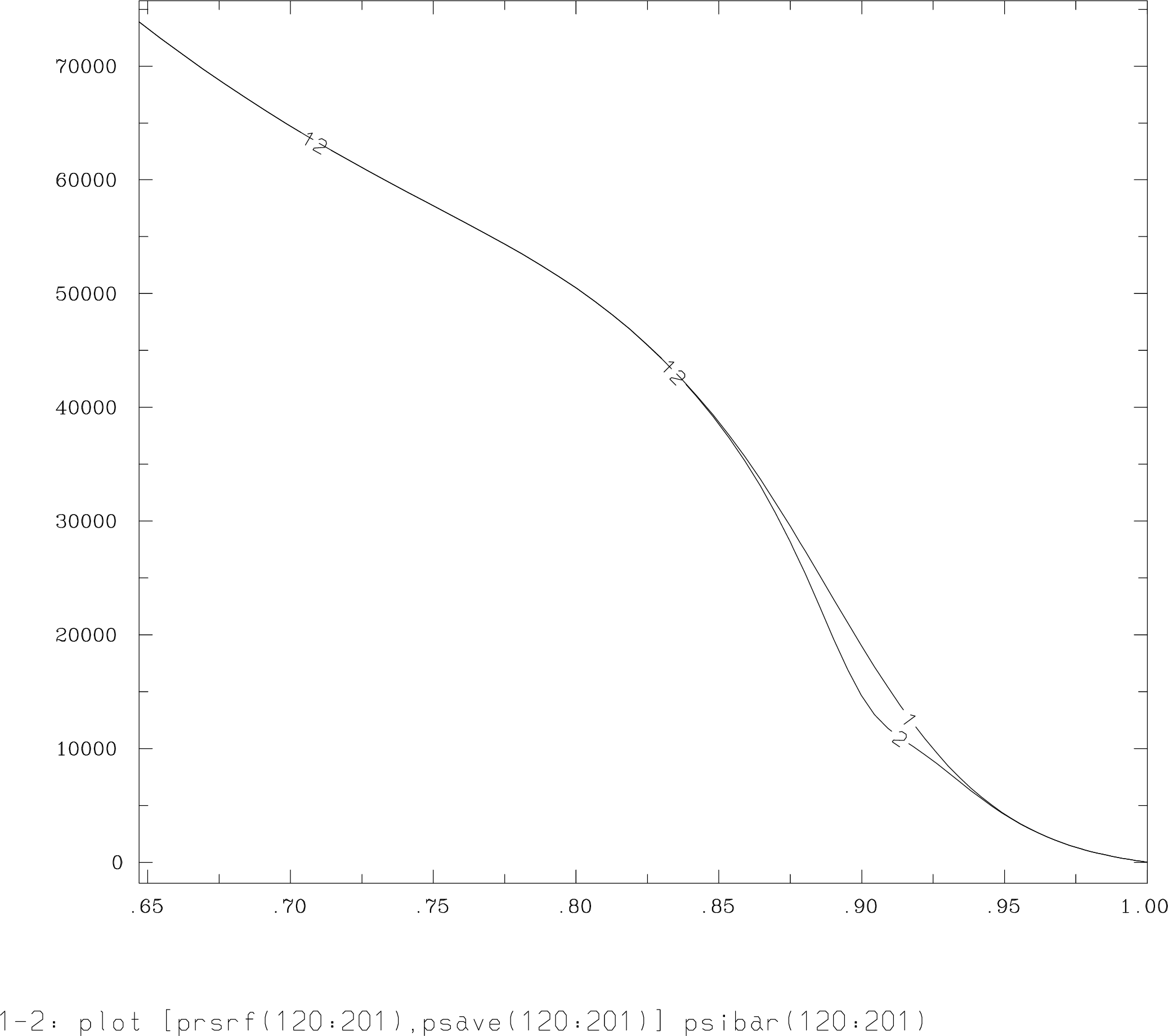
The MHD activity in this KSTAR experiment allows localizing the midpoint of the H-mode pedestal at approximately 222-223 cm of the major radius. The pedestal structure is not measured in this experiment. The line average density is found to be . Based on this information and typical KSTAR temperature profiles found in the KSTAR experiments, an unique solution for the equilibrium does not exist. Additional assumptions are needed. Stability analysis of equilibrium solutions might help to reduce the uncertainty. Here, I compare two sets of equilibria that are generated by Minwoo and myself. Minwoo used the Corsica code to generate the equilibrium. In order to match the midpoint of the H-mode pedestal with the experimental observations, he shifted the H-
mode pedestal to the region
away from the separatrix. The H-mode pedestal is localized in the range from 0.8 to 0.88 of the normalized poloidal flux. In order to maintain the line average density close to the experimental values, the density in the core has been increased. With the typical temperature profiles, the plasma pressure is somewhat peaked in the plasma core. The q value in the midpoint of the H-mode pedestal region is about 3.5. Because of moderate values of q and extended vacuum region between the H-mode pedestal and separatrix, this equilibrium is good for MHD stability analysis and for the extended MHD modeling.
The profiles for the plasma pressure, safety factor and parallel current density are shown below:

I have generated a second set of equilibria, using assumptions for the H-mode pedestal location that are based on the observations from other tokamaks such as DIII-D. The H-mode pedestal is localized from 0.95 to 1 of the normalized poloidal flux. The physical location of the H-mode pedestal midpoint is the same as in the Minwoo’s equilibria. The TOQ code has been used to generate these equilibria. The pedestal is located very close to the separatrix and the q value is relatively large in the midpoint of the H-mode pedestal (q~6.5). This equilibrium is more difficult to analyze because of large values of q profile. Also, the TOQ is the inverse equilibrium solver and analysis with the extended MHD codes will more difficult because the equilibrium does not include the vacuum region. It will be desirable to import the pressure profiles to the TEQ code in Corsica for coherent comparison of two sets of equilibria.
The profiles for the plasma pressure, safety factor and parallel current density for this equilibrium are shown below:

I have generated the stability diagram for the KSTAR discharge 7328. The DCON and ELITE codes were used. The finite toroidal mode numbers up to n=15 were included in the stability analysis.

The KSTAR equilibrium with an intentionally relaxed pedestal which is below the PB stability boundary (case# s13-t00-06) is studied using the XGC0 code.  There XGC0 simulations are performed to investigate the pedestal dynamics for different plasma collisionalities. The first case (xks1303) uses the density and temperature that are used to generate this equilibrium. 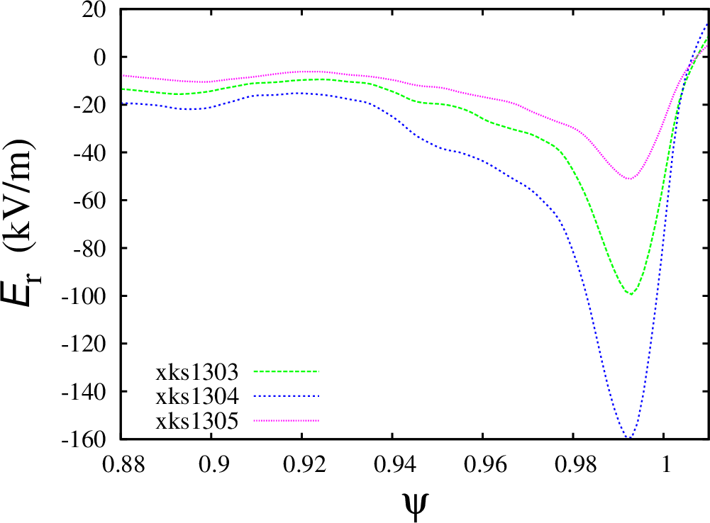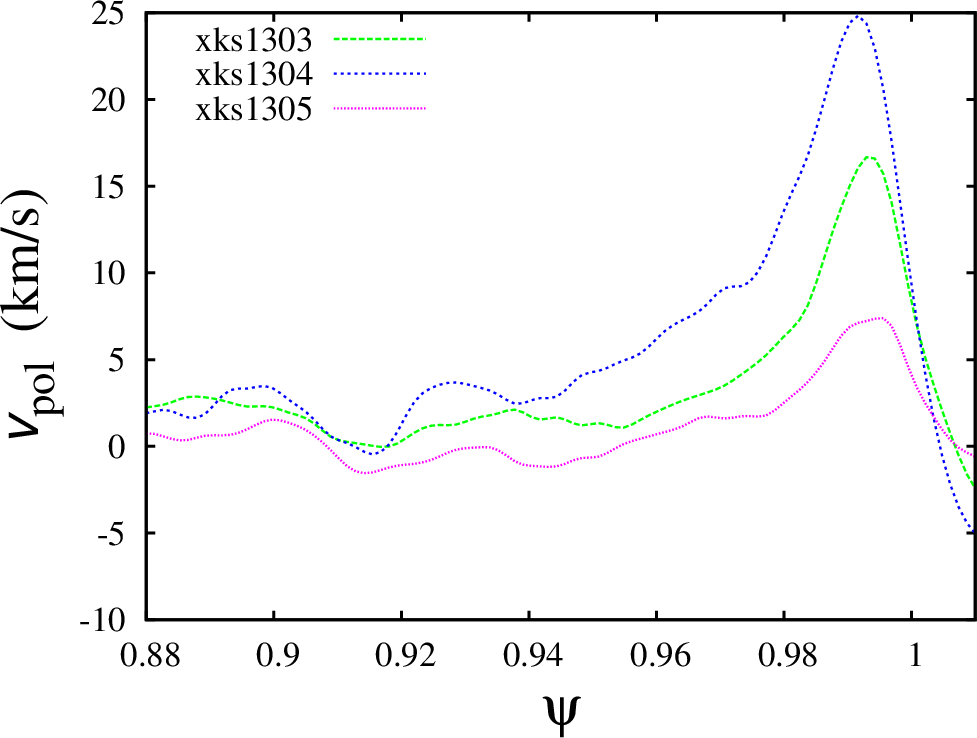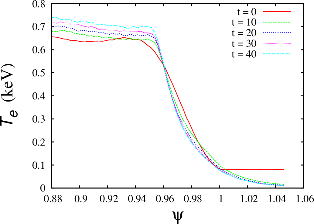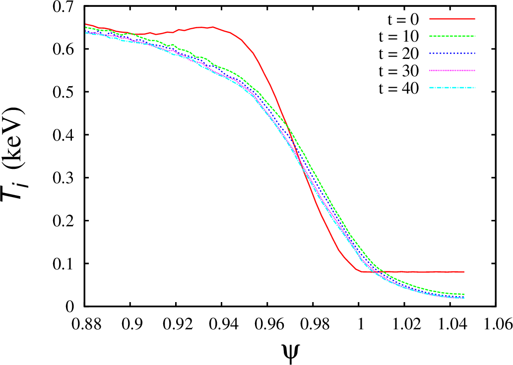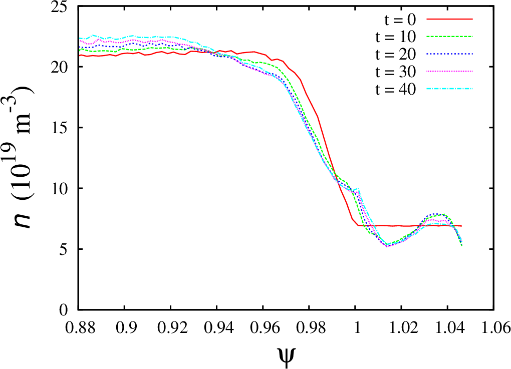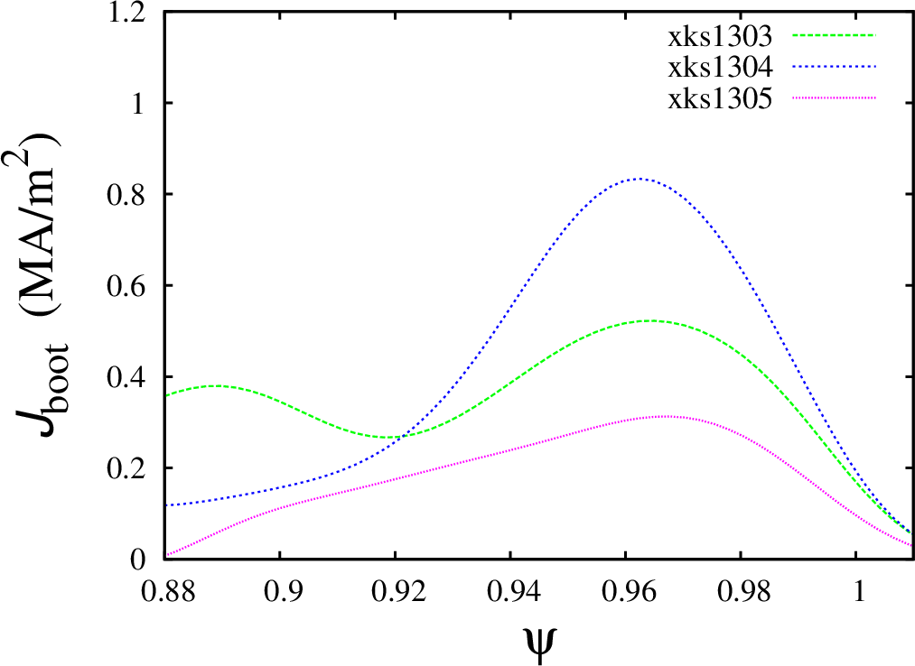The pedestal density is set to and the electron and ion temperatures are set to 500 eV. The pedestal temperature in two other XGC0 cases is varied slightly above the experimental error bars. The temperatures in the second case (xks1304) are set to 800 eV and temperatures in the third case (xks1305) are set to 300 eV. The density in these two cases are changes to keep the total plasma
pressure unchanged. The
density is set to  in the case xks1304 and to  in the case xks1305. The plasma collisionality for the case xks1304 is 4.38 times smaller than the plasma collisionality in the case xks1303 and the plasma collisionality in the case xks1305 is 4.63 times larger than the plasma collisionality in the case xks1303. The plasma collisionalities for the cases xks1305 and xks1304 differ by a factor of 20. Comparing the XGC0 results for the normalized plasma pressure that are given below, one can notice that the pedestal width is reducing for the low conditionality case.
Also, the pedestal height continue to grow at larger pace for the low collisionality case. This comparison can give a range of expected pedestal widths for the initial temperatures varied within experimental error bars.

There are significant differences in the bootstrap current predictions:

The bootstrap currents differ by a factor of 2.5 for these three cases that are still within the experimental error bars.

All XGC0 profiles are smoothed to remove the MC noise. Please note that the profiles continue to evolve and XGC0 simulations for these cases will be continued until quasi-steady states are obtained.

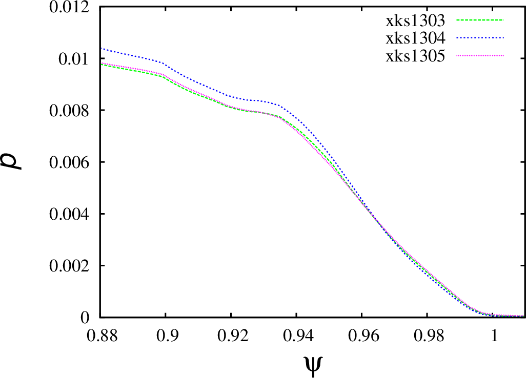
Based on I have created an initial equilibrium for the PB studies. In addition to the information in the Minwoo’s post, I have also used some information from our e-mail correspondence. In particular, I have set the line average density as and the central electron temperature as 1.3 keV. I have also made the following assumptions:

• The pedestal width is the same for the temperature and density profiles. It is equal to 0.06 of the normalized poloidal flux;
• The pedestal temperature is 400 eV;
• The pedestal density is ;
• The ion temperature is equal to the electron temperature;
• I assumed that the central q is slightly above unity.

I have also used relatively standard geometry parameters for KSTAR such as the major radius is 1.77 m, the minor radius is 0.47 m, elongation is 1.9, and triangularity is 0.8.

The q95 value that I am getting using the above settings is 5.06. The plasma pressure and q profiles are shown below.