Integrated Modeling of Tokamak Plasmas

In order to identify minimum MHD model sufficient for nonlinear MHD analysis of KSTAR discharges, the following models in the NIMROD code were considered:

1. Resistive MHD
   • Lundquist number
   • The Spitzer resistivity is used
   • No parallel viscosity or gyro-viscosity
   • No particle diffusivity, hyper-diffusivity or hyper-resistivity
2. Resistive MHD with drifts
   • Parallel viscosity and gyro-viscosity are enabled
   • Particle diffusivity is enabled
   • No hyper-diffusivity
3. Two-fluid MHD
4. Two-fluid two-temperature MHD

Equilibria generated for the BOUT++ stability analysis and provided by Minwoo have used in this NIMROD analysis.

The simulation results below are given for the equilibriun number #3 from the set of equilibria obtained from Minwoo Kim on August 31. The NIMROD grid in these simulation is 72×512 with polynomial degree of 6.

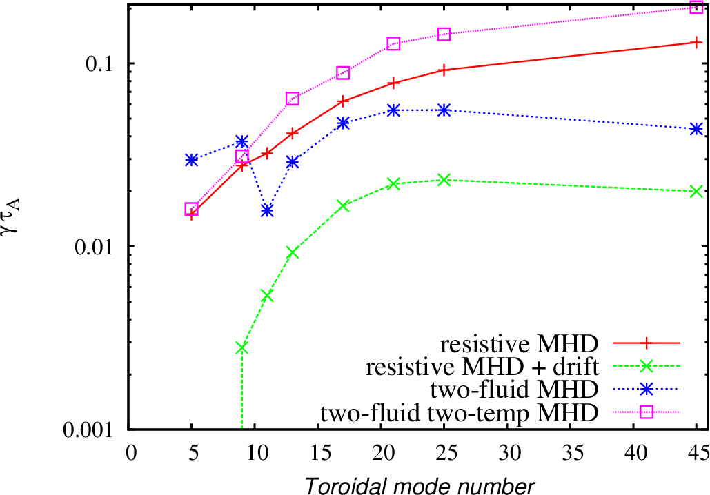
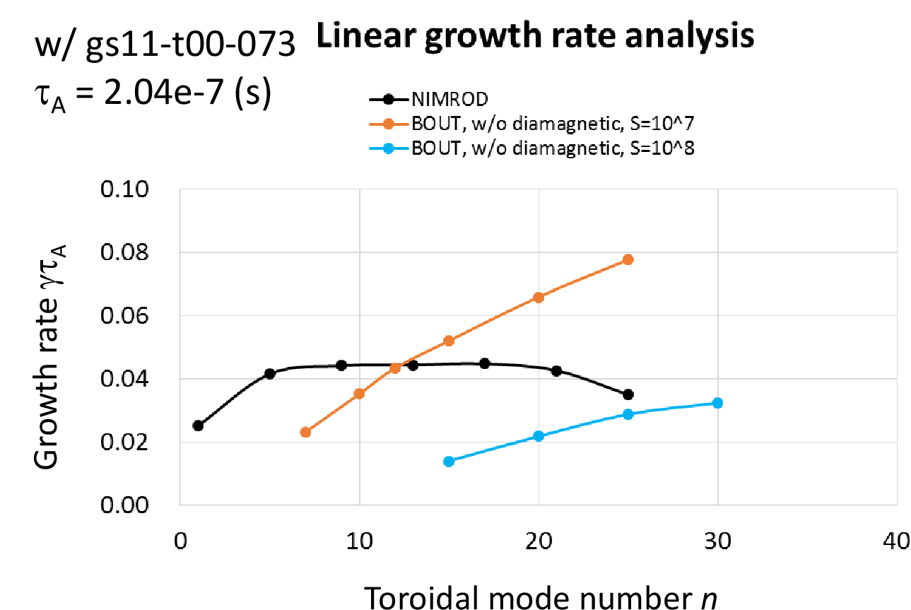
Normalized growth rates as functions of toroidal mode numbers.

The spectrum of the most unstable toroidal modes is different comparing to the predictions produced by Minwoo using the BOUT++ code. The ELM model that Minwoo uses in his simulations is somewhat similar to the restive MHD model with drifts in the NIMROD code. The NIMROD results are very moderately peaked around n=20-30, while the BOUT++ results showed the pecking for lower toroidal mode numbers. The two fluid results in NIMROD show better peaking for n=20-25. However, the modes remain rather unstable for n=45. The nonlinear simulations that would include first 45 toroidal modes might still be underresolved. For the two-fluid nonlinear NIMROD simulations, it is better to select equilibrium with the pressure profiles somewhat more relaxed in the H-mode pedestal region and with the larger bootstrap fraction so that lower n modes are more unstable.

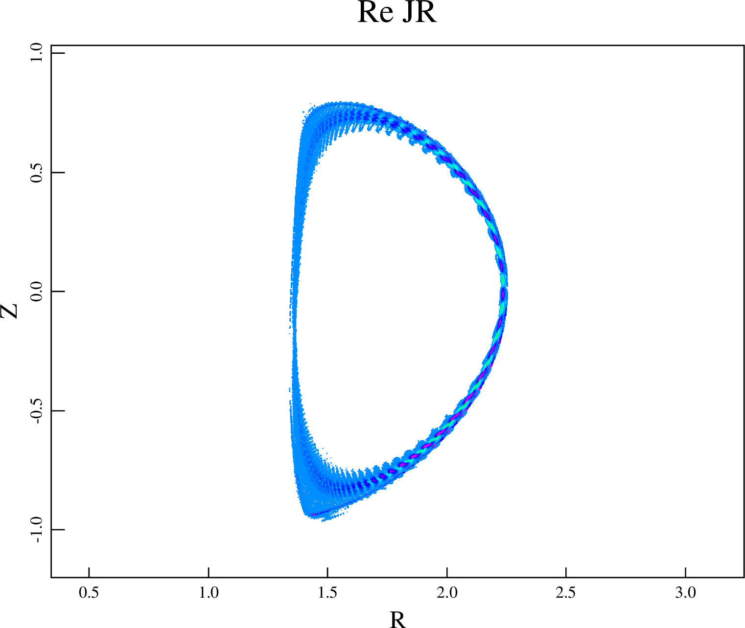
The eigenmode structure for low- and  high- toroidal mode numbers are found different in the two fluid simulations. The unstable lower toroidal mode numbers are found to be localized in the high filed side region, while the higher toroidal mode numbers are found to have more ballooning like nature. The transition between these two distinguishably different regions is found around n=9.

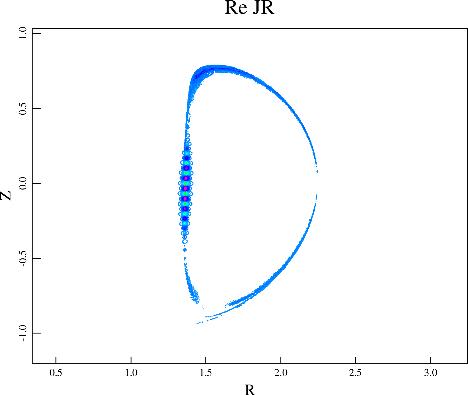
Mode structure for n=5

Mode structure for n=17.

The inclusion of two-temperature effects is found to affect the mode sprectrum and mode structure. The toroidal mode number of the most unstable modes is larger than the maximum toroidal mode number investigated in this study.

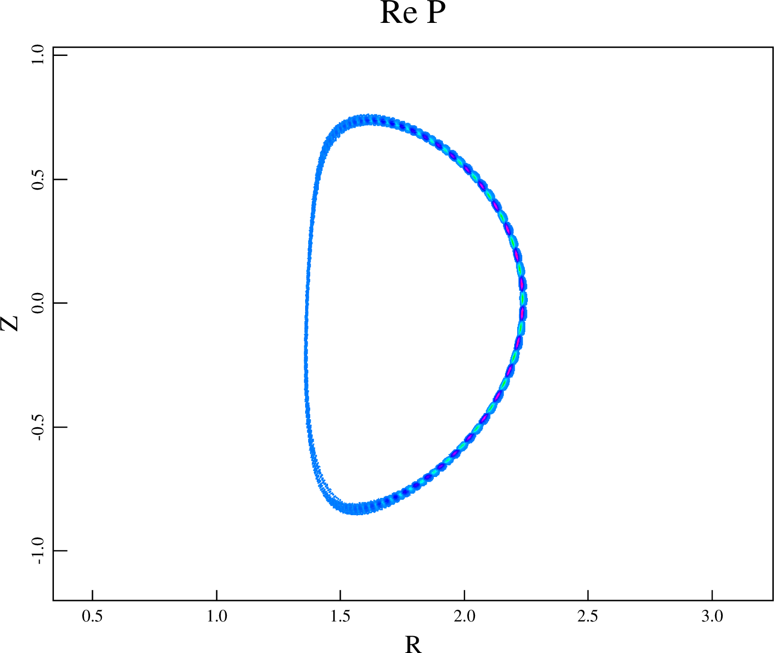
Pressure perturbations for n=17 found in the two-fluid NIMROD simulation.

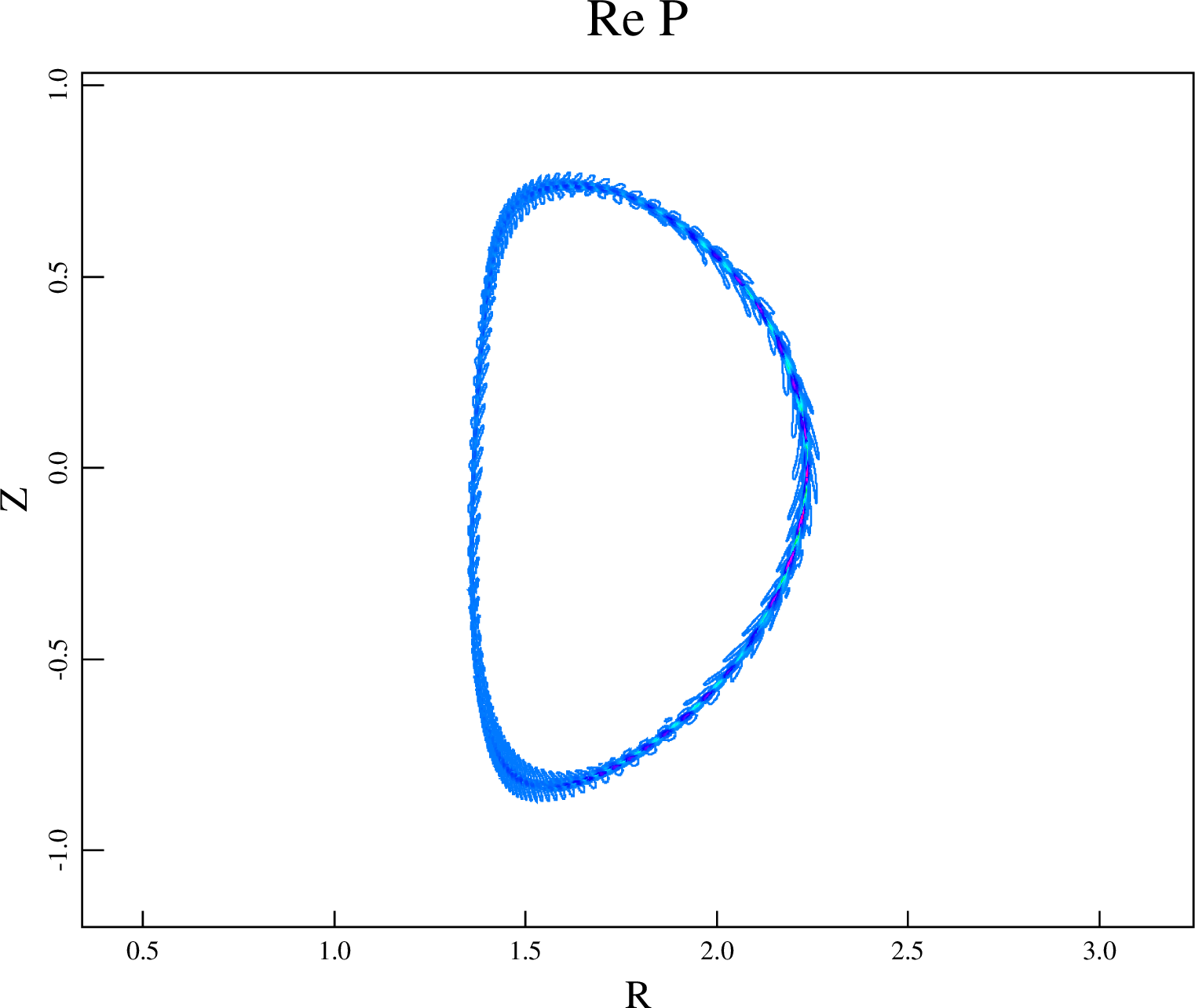
Pressure perturbations for n=17 found in the two-temperature two-fluid NIMROD simulation.

The modes found in the two-temperature NIMROD simulations are sight more shifted towards the pedestal top comparing to the modes found in the two-fluid simulations. It looks like that the inclusion of two-temperature effects destabilizes a different types of modes comparing to the modes found in the two-fluid simulations. In order to investigate the properties of these modes, the density profiles in the original equilibrium has been altered so that the density gradient in the pedestal region has been changed. The pressure profile is not affected by this change. The density width has been changed from 0.013 to 0.03 in this scan. In addition, the density at the separatrix has been increased to investigate how this change will effect the growth rates in two-temperature two-fluid simulations. Note that the resistivity in the density width scan remains modestly affected. However, the resistivity in the simulation with the increased separatrix density is strongly effected because the separatrix temperature has been reduced to keep the pressure profiles unchanged.

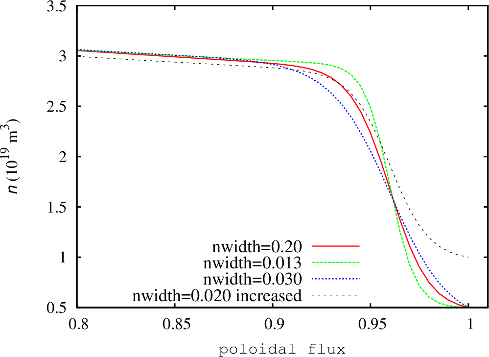
Pedestal density profiles.

The growth rates for the first three cases are found comparable to each other in the resistive MHD and two-fluid simulations. The growth rates for the fourth case are found significantly larger than the growth rates in three other cases in the resistive MHD NIMROD simulations. It is also found that the the increased density gradient result in lower growth rates in the two-temperature NIMROD simulations. Such behavior is typical for ITG modes that are destabilized when the ratio of temperature gradient to the density gradient is increased.

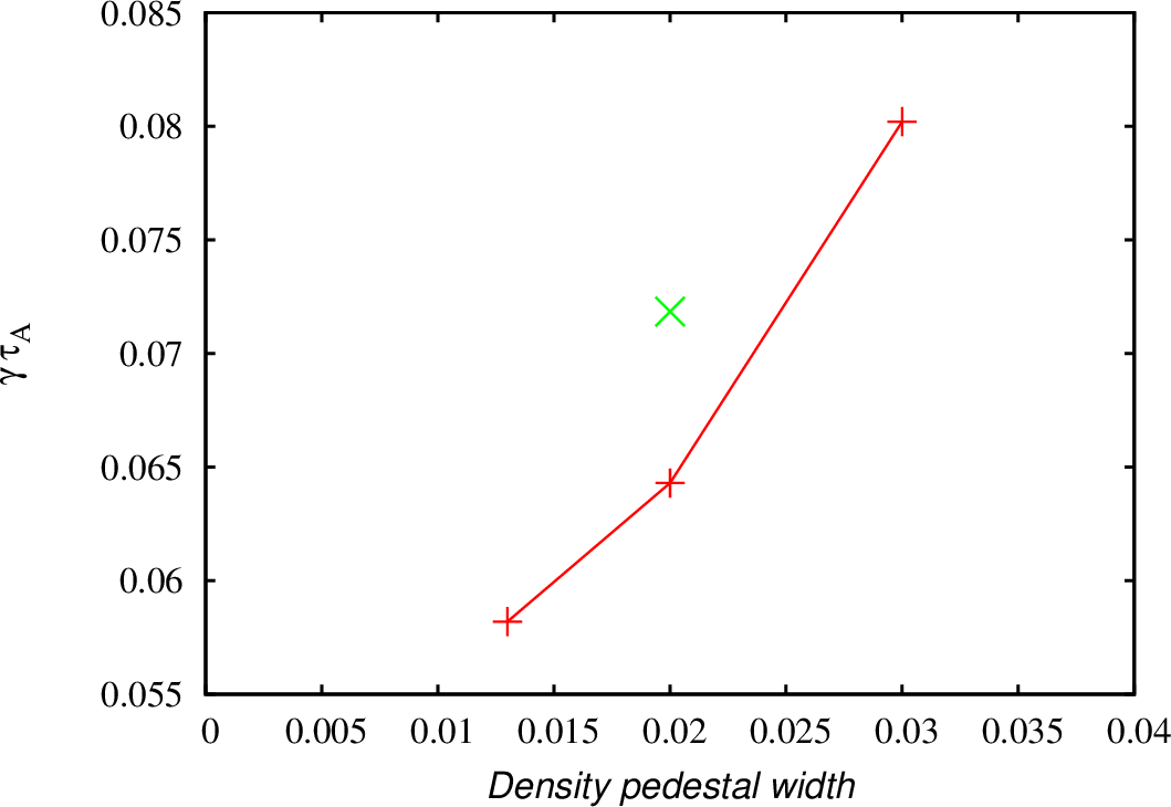
Normalized growth rates.

Minwoo has tested the equilibrium reconstruction procedure described in this post. He has noticed that the q-profile changes significantly when the direct solution is reconstructed from the inverse solution by the TEQ code. I can reproduce the Minwoo observations and confirm that the whole q-profile shifts by about 10% when the direct equilibrium is generated from the inverse equilibrium. It might be useful if the TEQ developers can address this problem. Meantime, I have modified the equilibrium reconstruction procedure to avoid the problem with the q-profile. In the modified procedure, we postpone the generation of the direct equilibrium until very last step:

caltrans 007328_4400.sav  -probname ss-test kstar.bas

thetac=1e-3; epsrk=5.e-9; nht=5000; start_inv
psave=...
teq_inv(0,1); teq_inv(0,1)

saveq("s13-t00-01.sav")

thetac=1e-3; epsrk=5.e-9; nht=5000; start_inv

qsave=...
teq_inv(0,1); teq_inv(0,1)

saveq("s13-t00-02.sav")

jparsave(81:101)=jparsave(80)

real ndens=psibar; ndens=2.6e19
real prbs=psave/10./2.
real tebs=prbs/ndens/1.602e-19
real zeffbs=psave; zeffbs=1.
real pbeambs=psibar; pbeambs=0.
read jbootstrap.bas

real jbs1 = jbootstrap(prbs,ndens,tebs,tebs,zeffbs, pbeambs, 1., 1., 0.)
real jbs0 = jbs1(:,1)
real foo1=tanh((1.01-psibar)/0.05)
real foo2=(1+tanh((psibar-0.7)/0.05))/2.
jparsave=jparsave*foo1+jbs0/bsqrf*foo2

thetac=1e-3; residj=1e-9; nht=5000; start_inv
jparsave=jparsave*foo1+jbs0/bsqrf*foo2
nf; plot [jparsrf,jparsave], asrf+rsrf
teq_inv(3,0); teq_inv(0,1); teq_inv(0,1)
inv_eq=0; inv_k=0; run
saveq("s13-t00-03.sav")

gridup; run; saveq("s13-t00-04.sav")

gridup; run; saveq("s13-t00-05.sav")

weqdsk

In the plasma core region, the q-profile is not affected now. In the plasma edge region, the q-profile is modified. However, these changes are consistent with the bootstrap current model. It looks that the bootstrap current fractions computed in TEQ and TOQ does not agree well. In order to reproduce the TOQ bootstrap current, a scaling factor for the parallel current density is needed.

An important progress in the understanding of the pedestal structure in the KSTAR discharge 7328 has been made during my visit. In particular:

1. A new procedure to generate free boundary equilibrium for KSTAR discharges has been developed. This procedure is documented and is available online.
   The improvements of the new equilibrium includes the following:
   1. The (R,Z) resolution has been increased by a factor of four. The stability analysis as well as extended MHD studies require well-resolved equilibrium;
   2. The central values of q has been reduced from 2 to more realistic values that takes into account episodic sawtooth crashes in this discharges;
   3. The pedestal is moved from the region (0.8:0.9) to (0.9:1);
   4. The densities and temperatures in the plasma core have more realistic values. Near the magnetic axis, the plasma pressure in the new equilibrium is significantly smaller comparing to the pressure in the old equilibrium;
   5. The new equilibria include vacuum field solutions and can be used for the nonlinear extended MHD studies of ELM crashes.
2. Using the new equilibrium (case s17), a new peeling-ballooning diagram is generated. The diagram is also described and available online. Key features of the PB diagram include:
   • The diagram indicates the toroidal mode numbers that are close to be modes observed in experiments. The modes identified on the PB diagram are n=5, n=9 and n=11;
   • Both the peeling and ballooning boundaries were identified;
   • The experimental pedestal conditions that are expected to correspond to n=5 and n=9 modes are determined;
   • It is indicated that transition from n=9 to n=5 modes is likely to be associated with very small changes in the pedestal density and temperature, but rather significant changes in the parallel current density;
   • The pedestal temperatures that are found to be associated with n=5 and n=9 are 800 eV and 775 eV correspondingly. These values are somewhat above the experimental temperatures that are expected to be in the range from 400 eV to 700 eV. The differences between temperature found in the stability analysis and experimental range for temperatures can be explained if the Sauter model, that has been used in this analysis for the bootstap current, over-predicts the values of the bootstrap current. The expected over-predict is about 20%.
3. The kinetic neoclassical XGC0 code has been used to investigate the pedestal buildup dynamics. For this study, a KSTAR equilibrium with somewhat relaxed pedestal has been used. The results of this study are documented here and here.
   • For the range of expected temperatures, it is noted that the pedestal buildup dynamics can be very different. The cases with lower plasma collisionality exhibit a faster pedestal buildup. For these case, the pedestal height is increasing and the pedestal width is decreasing faster comparing to the cases with higher plasma collisionality. The cases with lower collisionality are likely to be become unstable sooner for the PB modes.
   • The kinetic predictions for the bootstrap currents are compared for these case. It is shown that the bootstrap current is significantly larger for the cases with lower plasma collisionality. Similar observations are made for the radial electric field and the poloidal velocity rotation profiles.
4. The extended MHD simulations of the KSTAR discharge 7328 using the NIMROD and BOUT++ codes are compared here. It has been shown that
   • The NIMROD and BOUT++ produce comparable growth rates;
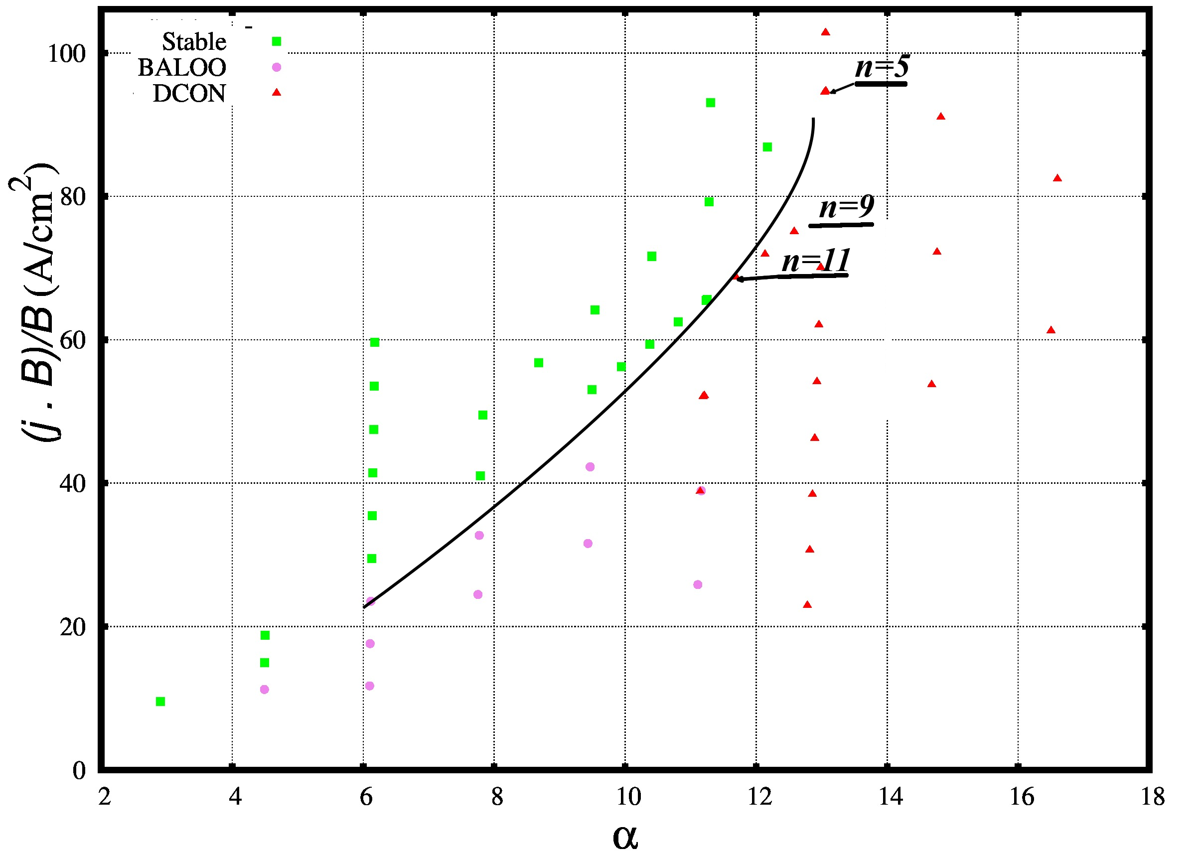
   • The resistivity profiles and a proper account for the diamagnetic effects are important;
   • The parallel viscosity effects have relatively weak effect on the ELM dynamics at least during a linear stage of a crash.

Possible future studies can include:

• Improvements in the equilibrium solve in the vacuum region and further increase in the (R,Z) resolutions;
• Verification and validation of the bootstrap current models. It will be interesting to confirm one of the conclusions from the PB stability analysis that the Sauter model over-predicts the bootstrap currents in the KSTAR pedestal. The expected over-predict can be of order of 20%. The XGC0 code or some other new models for the bootstrap current can be compared with Sauter.
• The XGC0 simulations with impurities can be performed to compare with the available experimental measurements from KSTAR including rotation profiles etc.
• Comparison of NIMROD and BOUT++ results can be continued. The objective of this study can be the development of extended MHD model that includes necessary and essential physics to describe ELM. The importance of various two-fluid and FLR effects are still needs to be confirmed for the KSTAR plasma parameters. It is not completely clear if separate evolution of density will change linear or nonlinear results. Finally, the nonlinear dynamics of ELMs and the propagation of ELM filaments to the plasma wall including the associated heat loads can be investigated. As a near term objective of this NIMROD/BOUT++ study can be a test of hypothesis that the two-fluid effects nearly cancel the resistivity effects, and ideal stability analysis can be used for KSTAR.

The stability analysis of the KSTAR discharge 7328 is presented below. The initial settings for this study are based on the pedestal parameters and other plasma parameters that are outlined in the case s17.

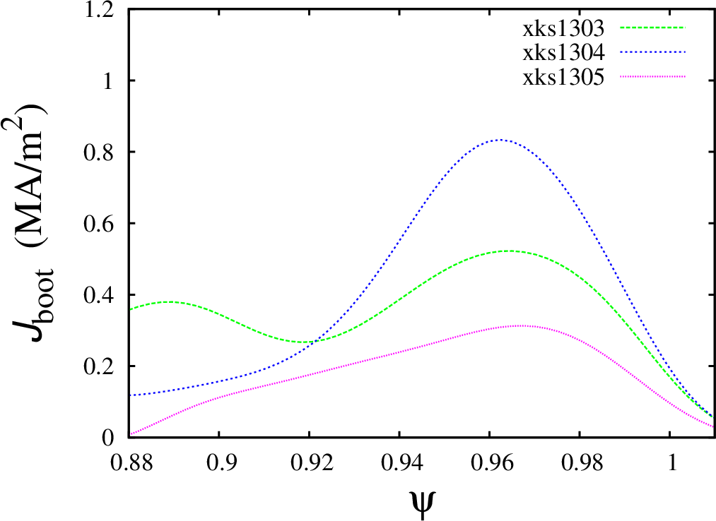
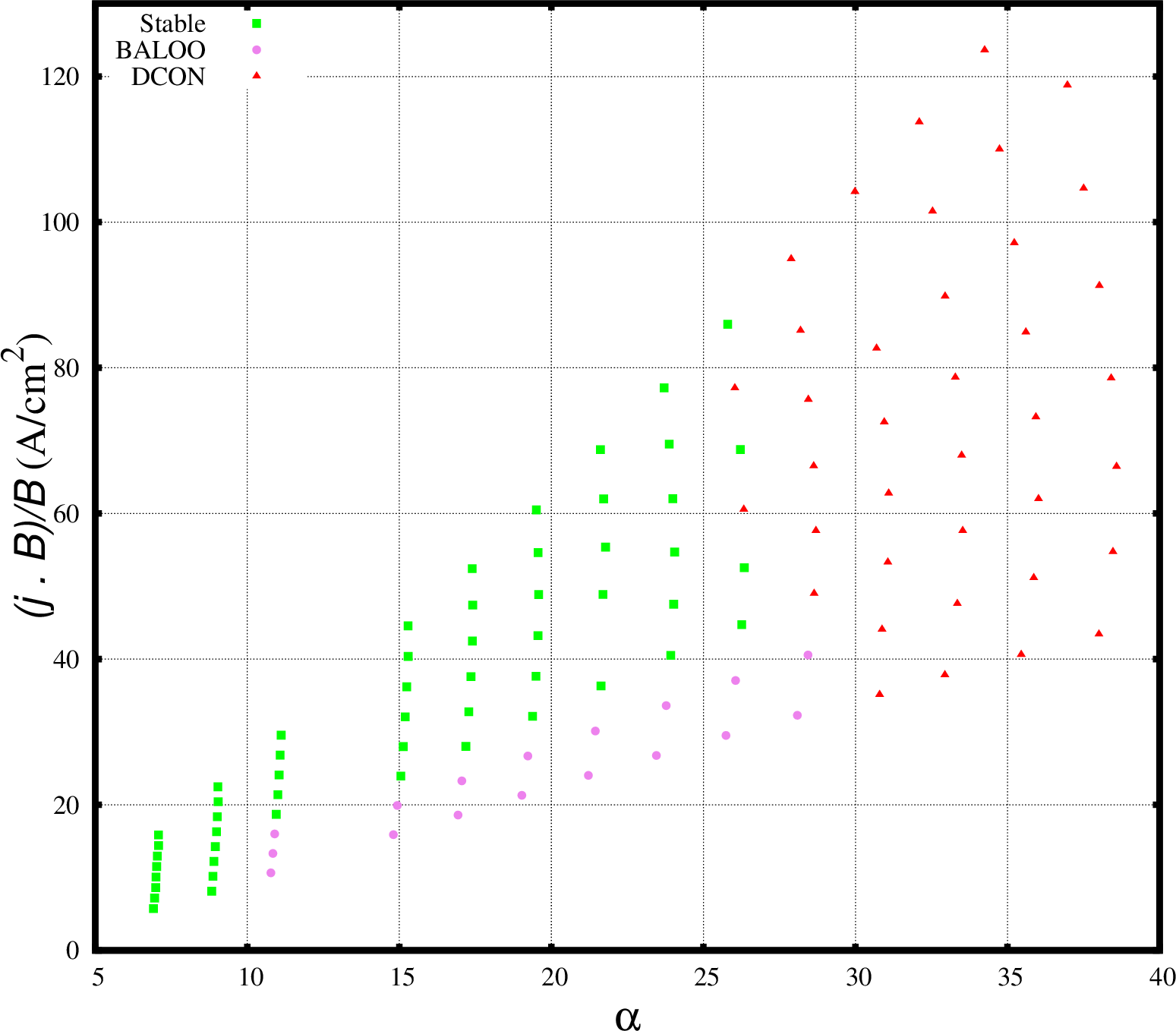
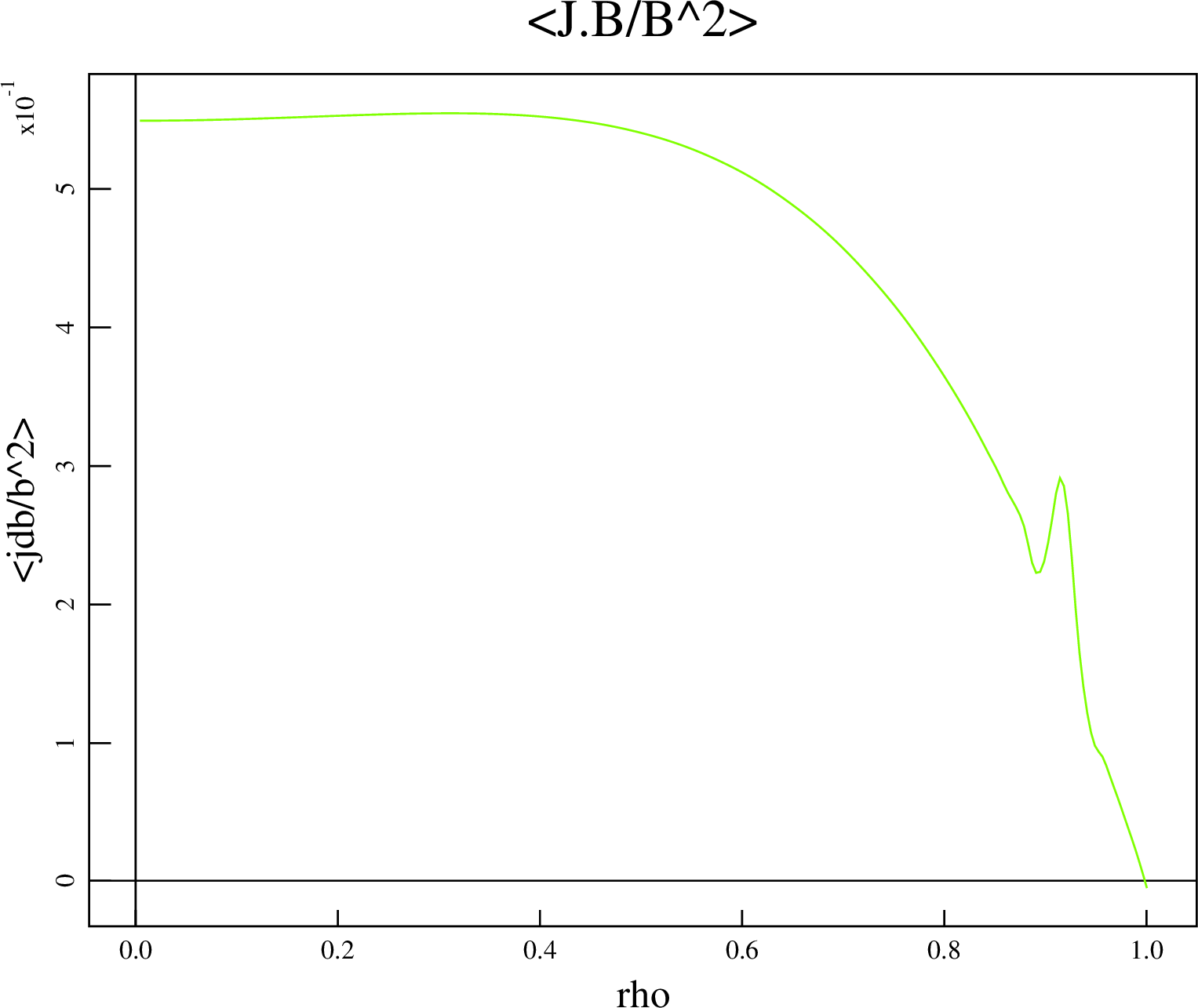
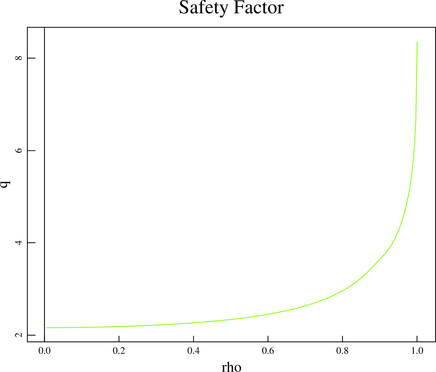
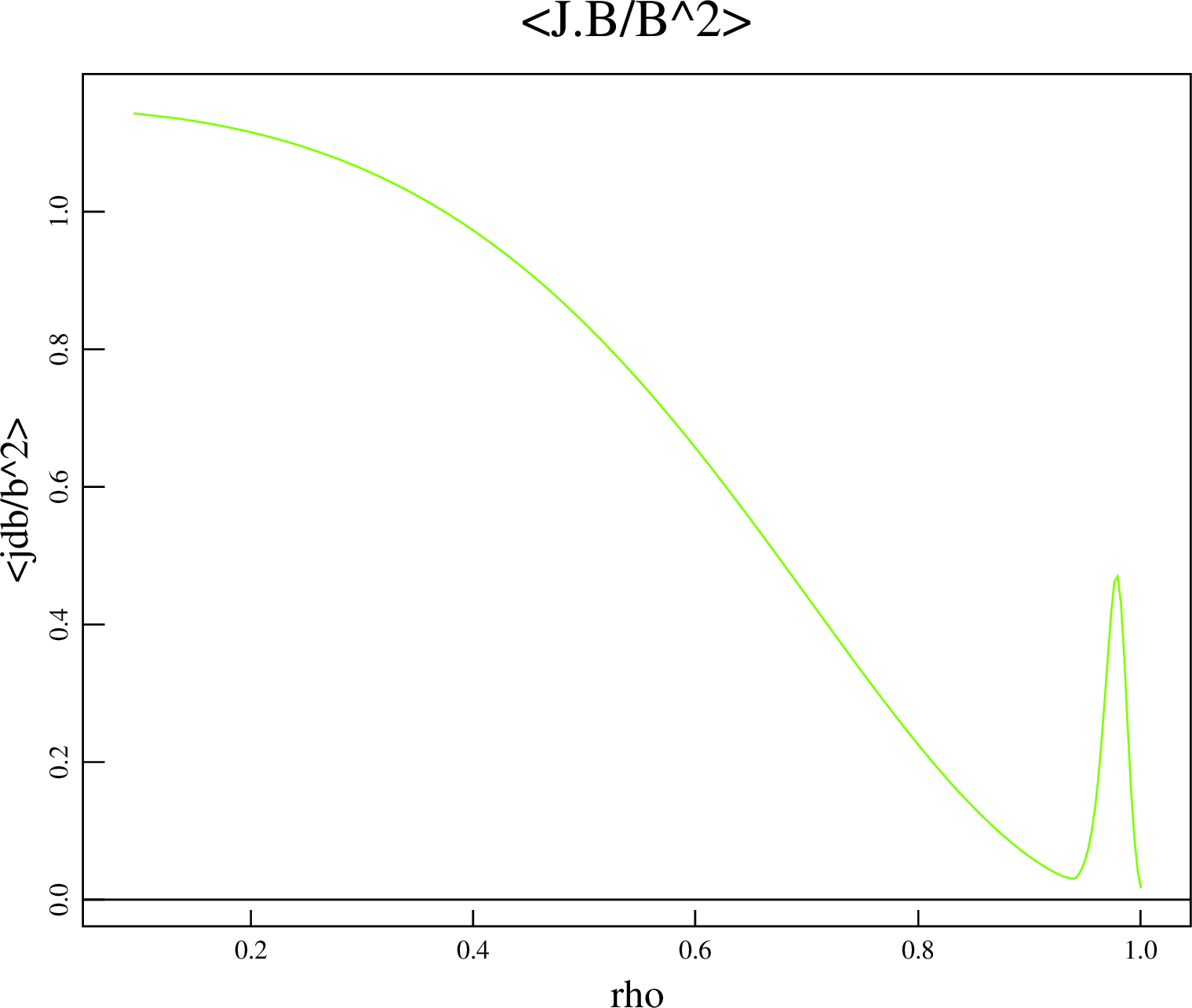
The ballooning stability boundary is shown on this plot. The peeling stability boundary is also identified. However, the parallel current density that will make the peeling modes unstable are significantly large and are in the range of . The and toroidal mode numbers that are close to the experimentally observed modes are marked on the diagram. Note, the transition from to will be associated with very small changes in the normalized plasma density and with relatively large changes in the parallel current density. The pedestal plasma density for both equilibria was , the pedestal temperatures were and for the cases of and unstable modes correspondingly. The bootstrap current was computed using the Sauter formula for the case of mode and using the Sauter formula with the scaling factor of 1.2 for the case of mode.

If the values of the plasma temperatures is on the upper boundary of the experimental error bar (or slightly above the error bar), the likely conclusion is that the Sauter formula for KSTAR pedestal parameters under-predicts the bootstrap current.

The XGC0 code has been also used to model the radial electric field and poloidal velocity profiles for the KSTAR discharge 7328. The profiles for the three cases with different collisionalities that are described in the previous post are shown below.

Radial electric field (outside midplane)

Poloidal velocity profiles

The poloidal velocity and radial electric field in the H-mode pedestal region strongly depend on the plasma collisionality.

NIMROD and BOUT++ results are compared for the case gs11-t00-t073 that is generated using the procedure described in the previous post. The growth rates computed using the NIMROD and BOUT++ codes are compared below.

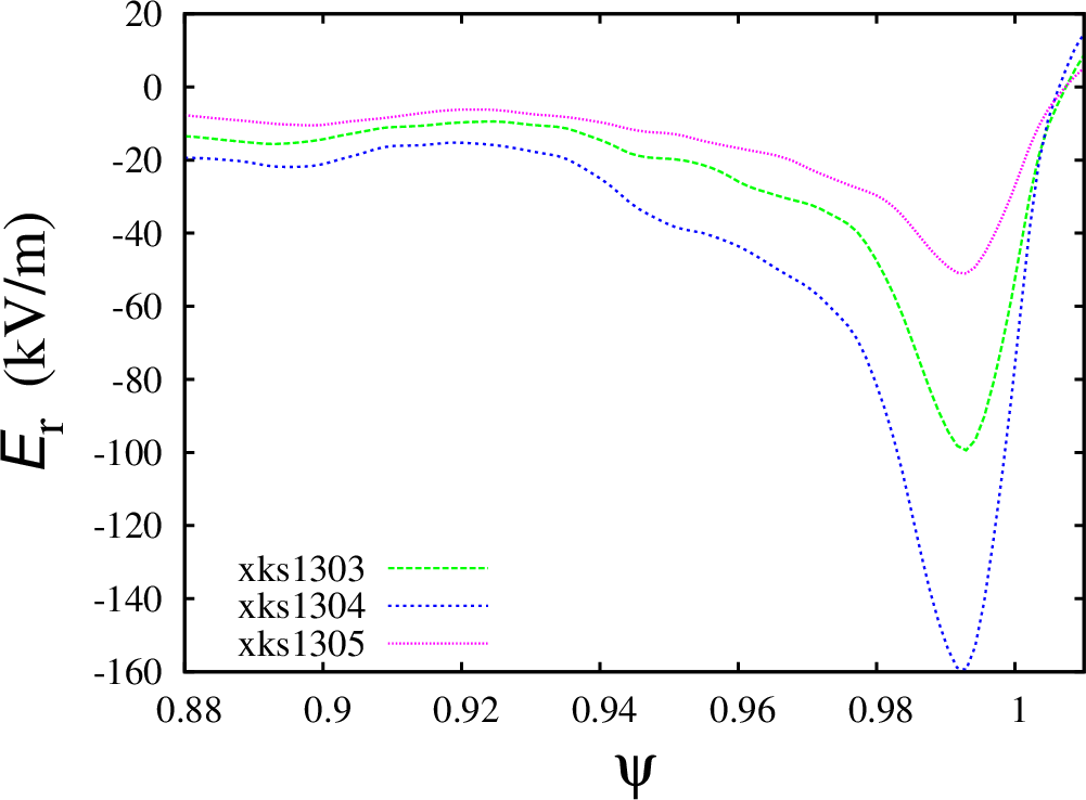
The NIMROD results and BOUT++ results that are shown as blue curve are run with . However, the constant resistivity profile is used in these simulations. There are several conclusions from these and other NIMROD/BOUT++ comparison simulations:

1. The resistivity profiles and a proper account for the diamagnetic effects are important;
2. The parallel viscosity effects have relatively weak effect on the ELM dynamics at least during a linear stage of a crash.

The following steps are used for KSTAR equilibrium reconstruction:

1. Generate a new inverse equilibrium using the TOQ equilibrium solver. There are certain assumptions for the plasma profiles in the process. In particular, the case s13-t00-06 uses these parameters for the plasma profiles:

    modelp=27
    nedge13=0.7
    nped13=2.6
    ncore13=4.6
    nexpin=1.1
    nexpout=1.1
    tedgeEV=70.
    tpedEV= 500
    tcoreEV=2600.0
    texpin=1.1
    texpout=2. 
    widthp=.07
    xphalf=.91

2. The DCON stability code is used the test the stability of resulting equilibrium
3. The plasma profiles from TOQ are interpolated to the TEQ grid in Corsica. These profile include the plasma pressure and safefy factor.
4. The interpolated plasma pressure and the interpolated safety factor are sent to TEQ to generated new geqdsk files that would include the vacuum field solution.
   The Corsica psave and qsave variables are used.
   • We start with the original sav-file for this discharge: 

     caltrans 007328_4400.sav  -probname ss-test kstar.bas

   • Then, we update the pressure profile and generate new inverse solution:

     thetac=1e-3; epsrk=5.e-9; nht=5000; start_inv
     psave( 1: 26)=[4.0652e+05,4.0636e+05,4.0589e+05,4.0510e+05,4.0400e+05,4.0259e+05,4.0085e+05,3.9876e+05,3.9636e+05,3.9354e+05,3.9038e+05,3.8681e+05,3.8290e+05,3.7861e+05,3.7397e+05,3.6897e+05,3.6364e+05,3.5798e+05,3.5201e+05,3.4573e+05,3.3917e+05,3.3235e+05,3.2528e+05,3.1798e+05,3.1047e+05,3.0278e+05]
     psave( 27: 52)=[2.9493e+05,2.8693e+05,2.7881e+05,2.7061e+05,2.6233e+05,2.5400e+05,2.4565e+05,2.3729e+05,2.2897e+05,2.2067e+05,2.1246e+05,2.0432e+05,1.9630e+05,1.8841e+05,1.8065e+05,1.7307e+05,1.6566e+05,1.5845e+05,1.5144e+05,1.4466e+05,1.3810e+05,1.3179e+05,1.2572e+05,1.1991e+05,1.1436e+05,1.0907e+05]
     psave( 53: 78)=[1.0405e+05,9.9302e+04,9.4818e+04,9.0599e+04,8.6643e+04,8.2945e+04,7.9499e+04,7.6298e+04,7.3334e+04,7.0596e+04,6.8068e+04,6.5736e+04,6.3577e+04,6.1565e+04,5.9667e+04,5.7842e+04,5.6037e+04,5.4183e+04,5.2207e+04,5.0025e+04,4.7558e+04,4.4737e+04,4.1586e+04,3.8103e+04,3.4179e+04,2.9900e+04]
     psave( 79:101)=[2.5535e+04,2.1282e+04,1.7332e+04,1.3874e+04,1.0920e+04,8.4769e+03,6.5566e+03,5.0422e+03,3.8616e+03,2.9488e+03,2.2444e+03,1.6993e+03,1.2741e+03,9.5421e+02,7.0459e+02,5.0154e+02,3.5481e+02,2.3120e+02,1.4798e+02,8.3140e+01,3.6807e+01,8.9772e+00,3.4489e+00]
     teq_inv(0,1); teq_inv(0,1)

     The inverse equilibrium solver is called with the options to keep the plasma current unaltered. We run the solver two times, because the solver has a tendency to inverse the plasma current in the equilibrium solution.

   • Then, the direct solution is generated using direct TEQ solver:

     inv_eq=0; inv_k=0; run

   • The solution is stored in a new sav-file

     saveq("s13-t00-01.sav")

   • The q-prifiles are being updated now:

     thetac=1e-3; epsrk=5.e-9; nht=5000; start_inv

     qsave( 1: 26)=[1.3999e+00,1.4000e+00,1.4006e+00,1.4014e+00,1.4026e+00,1.4041e+00,1.4060e+00,1.4082e+00,1.4108e+00,1.4137e+00,1.4170e+00,1.4207e+00,1.4248e+00,1.4292e+00,1.4341e+00,1.4394e+00,1.4451e+00,1.4513e+00,1.4579e+00,1.4650e+00,1.4726e+00,1.4806e+00,1.4892e+00,1.4983e+00,1.5079e+00,1.5181e+00]
     qsave( 27: 52)=[1.5289e+00,1.5403e+00,1.5524e+00,1.5650e+00,1.5784e+00,1.5924e+00,1.6072e+00,1.6227e+00,1.6390e+00,1.6560e+00,1.6740e+00,1.6927e+00,1.7124e+00,1.7331e+00,1.7546e+00,1.7773e+00,1.8009e+00,1.8257e+00,1.8515e+00,1.8786e+00,1.9070e+00,1.9366e+00,1.9675e+00,1.9998e+00,2.0336e+00,2.0689e+00]
     qsave( 53: 78)=[2.1059e+00,2.1445e+00,2.1848e+00,2.2270e+00,2.2711e+00,2.3171e+00,2.3653e+00,2.4157e+00,2.4684e+00,2.5236e+00,2.5813e+00,2.6418e+00,2.7051e+00,2.7715e+00,2.8411e+00,2.9142e+00,2.9910e+00,3.0719e+00,3.1572e+00,3.2472e+00,3.3424e+00,3.4432e+00,3.5509e+00,3.6655e+00,3.7876e+00,3.9196e+00]
     qsave( 79:101)=[4.0602e+00,4.2122e+00,4.3736e+00,4.5492e+00,4.7362e+00,4.9360e+00,5.1541e+00,5.3890e+00,5.6429e+00,5.9183e+00,6.2180e+00,6.5436e+00,6.8934e+00,7.2872e+00,7.7253e+00,8.1641e+00,8.6979e+00,9.1615e+00,9.8188e+00,1.0331e+01,1.0697e+01,1.0917e+01,1.0960e+01]
     teq_inv(0,1); teq_inv(0,1)

   • New direct solution is generated again. The solution will include the update plasma pressure and q profiles:

     inv_eq=0; inv_k=0; run

     saveq("s13-t00-02.sav")

   • Now, we need to ensure that the bootstrap current is properly included. In order to do this, we will exclude the edge current from the jparsrf and will replace it with the bootstrap current from the Sauter model:

     jparsave(81:101)=jparsave(80)

     real ndens=psibar; ndens=2.6e19
     real prbs=psave/10./2.
     real tebs=prbs/ndens/1.602e-19
     real zeffbs=psave; zeffbs=1.
     real pbeambs=psibar; pbeambs=0.
     read jbootstrap.bas

     real jbs1 = jbootstrap(prbs,ndens,tebs,tebs,zeffbs, pbeambs, 1., 1., 0.)
     real jbs0 = jbs1(:,1)
     real foo1=tanh((1.01-psibar)/0.05)
     real foo2=(1+tanh((psibar-0.7)/0.05))/2.
     jparsave=jparsave*foo1+jbs0/bsqrf*foo2

   • Run a sequence of inverse and direct equilibrium solvers ensuring the the plasma current does not change:

     thetac=1e-3; residj=1e-9; nht=5000; start_inv
     jparsave=jparsave*foo1+jbs0/bsqrf*foo2
     nf; plot [jparsrf,jparsave], asrf+rsrf
     teq_inv(3,0); teq_inv(0,1); teq_inv(0,1)
     inv_eq=0; inv_k=0; run
     saveq("s13-t00-03.sav")

   • Increase the resolution in the direct equilibrium solution to 257×257 (at least):

     gridup; run; saveq("s13-t00-04.sav")

     gridup; run; saveq("s13-t00-05.sav")

   • Save the new geqdsk file

     weqdsk

   • Note, the the resolution for the inverse solver is also important and it might be useful to increase it by changing the values of map and msrf (theta and psi dimensions in the inverse solve) and running the inverse solver.
5. The new geqdsk can be used in the MHD stability codes or with extended MHD codes for further analysis. In order to modify this equilibrium even further, one can modify the pressure profile and parallel current density profile using the last sav-file. An example  below shows how to change the slope in the H-mode pedestal without changing the pedestal width:

    thetac=1e-3; epsrk=5.e-9; nht=5000; start_inv
    real foo2=(1+tanh((psibar-0.90)/0.02))/2.
    real foo1=(1-tanh((psibar-0.91)/0.02))/2.
    psave=prsrf*(2-(foo1+foo2))
    teq_inv(0,1); teq_inv(0,1)
    inv_eq=0; inv_k=0; run
    saveq("s13-t01-01.sav"); weqdsk

   Changes in the plasma pressure are shown below:
   

6. The final layout looks as shown:
   

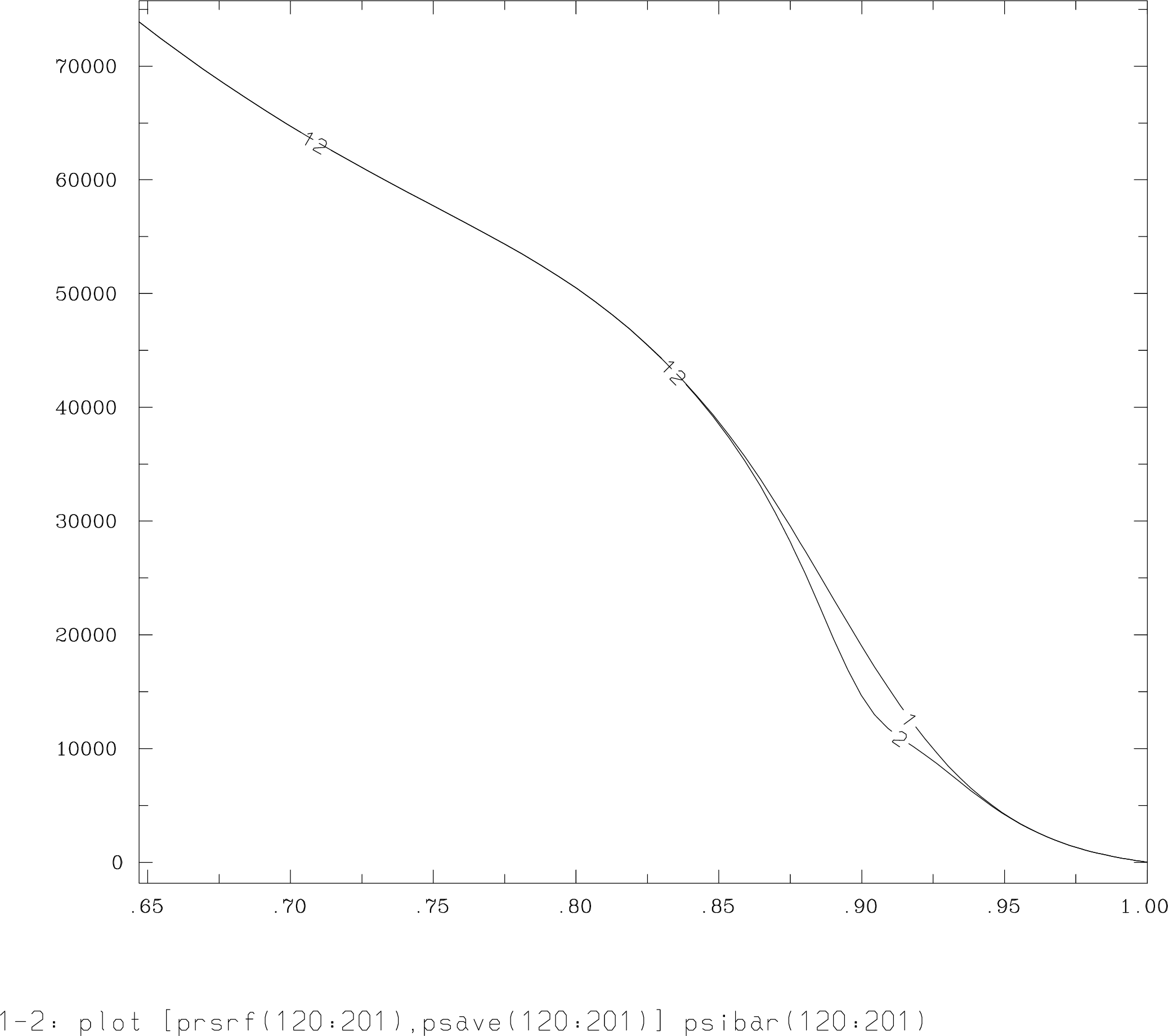
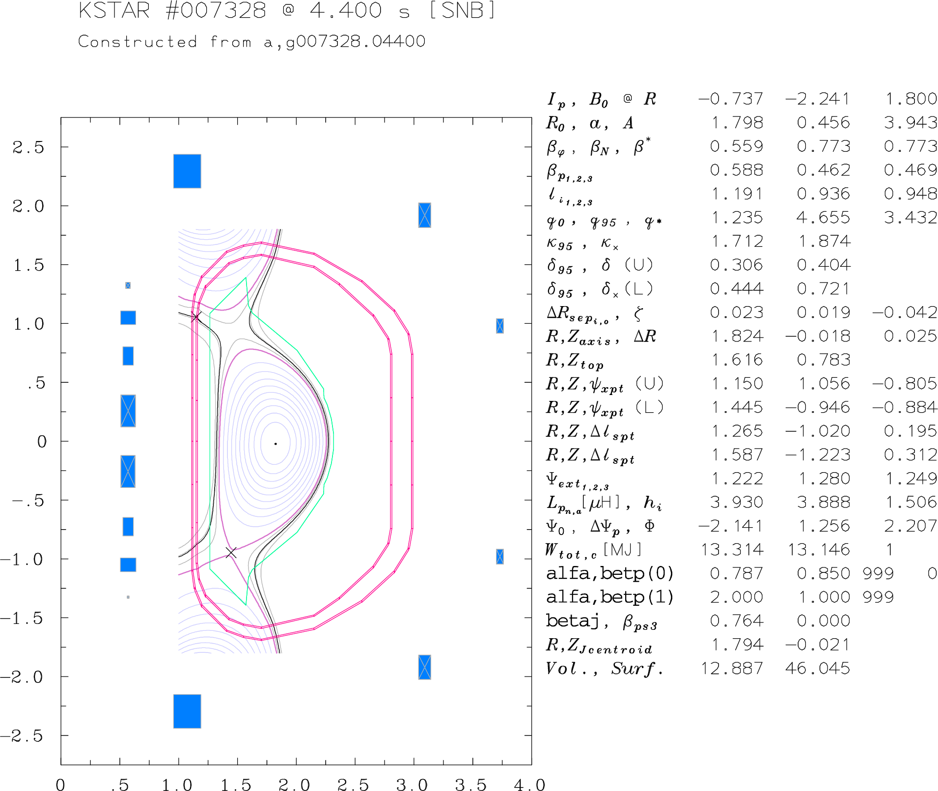
The MHD activity in this KSTAR experiment allows localizing the midpoint of the H-mode pedestal at approximately 222-223 cm of the major radius. The pedestal structure is not measured in this experiment. The line average density is found to be . Based on this information and typical KSTAR temperature profiles found in the KSTAR experiments, an unique solution for the equilibrium does not exist. Additional assumptions are needed. Stability analysis of equilibrium solutions might help to reduce the uncertainty. Here, I compare two sets of equilibria that are generated by Minwoo and myself. Minwoo used the Corsica code to generate the equilibrium. In order to match the midpoint of the H-mode pedestal with the experimental observations, he shifted the H-
mode pedestal to the region
away from the separatrix. The H-mode pedestal is localized in the range from 0.8 to 0.88 of the normalized poloidal flux. In order to maintain the line average density close to the experimental values, the density in the core has been increased. With the typical temperature profiles, the plasma pressure is somewhat peaked in the plasma core. The q value in the midpoint of the H-mode pedestal region is about 3.5. Because of moderate values of q and extended vacuum region between the H-mode pedestal and separatrix, this equilibrium is good for MHD stability analysis and for the extended MHD modeling.
The profiles for the plasma pressure, safety factor and parallel current density are shown below:

I have generated a second set of equilibria, using assumptions for the H-mode pedestal location that are based on the observations from other tokamaks such as DIII-D. The H-mode pedestal is localized from 0.95 to 1 of the normalized poloidal flux. The physical location of the H-mode pedestal midpoint is the same as in the Minwoo’s equilibria. The TOQ code has been used to generate these equilibria. The pedestal is located very close to the separatrix and the q value is relatively large in the midpoint of the H-mode pedestal (q~6.5). This equilibrium is more difficult to analyze because of large values of q profile. Also, the TOQ is the inverse equilibrium solver and analysis with the extended MHD codes will more difficult because the equilibrium does not include the vacuum region. It will be desirable to import the pressure profiles to the TEQ code in Corsica for coherent comparison of two sets of equilibria.
The profiles for the plasma pressure, safety factor and parallel current density for this equilibrium are shown below:

I have generated the stability diagram for the KSTAR discharge 7328. The DCON and ELITE codes were used. The finite toroidal mode numbers up to n=15 were included in the stability analysis.

The KSTAR equilibrium with an intentionally relaxed pedestal which is below the PB stability boundary (case# s13-t00-06) is studied using the XGC0 code.  There XGC0 simulations are performed to investigate the pedestal dynamics for different plasma collisionalities. The first case (xks1303) uses the density and temperature that are used to generate this equilibrium. 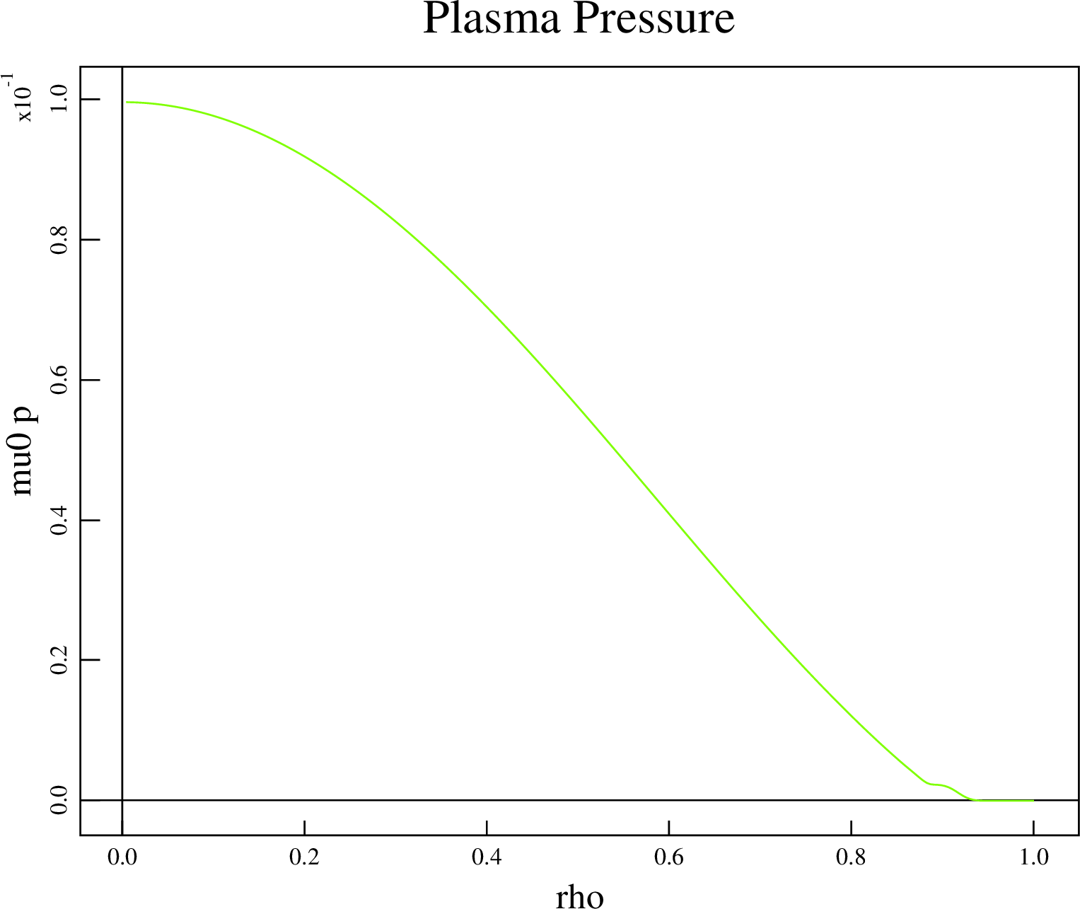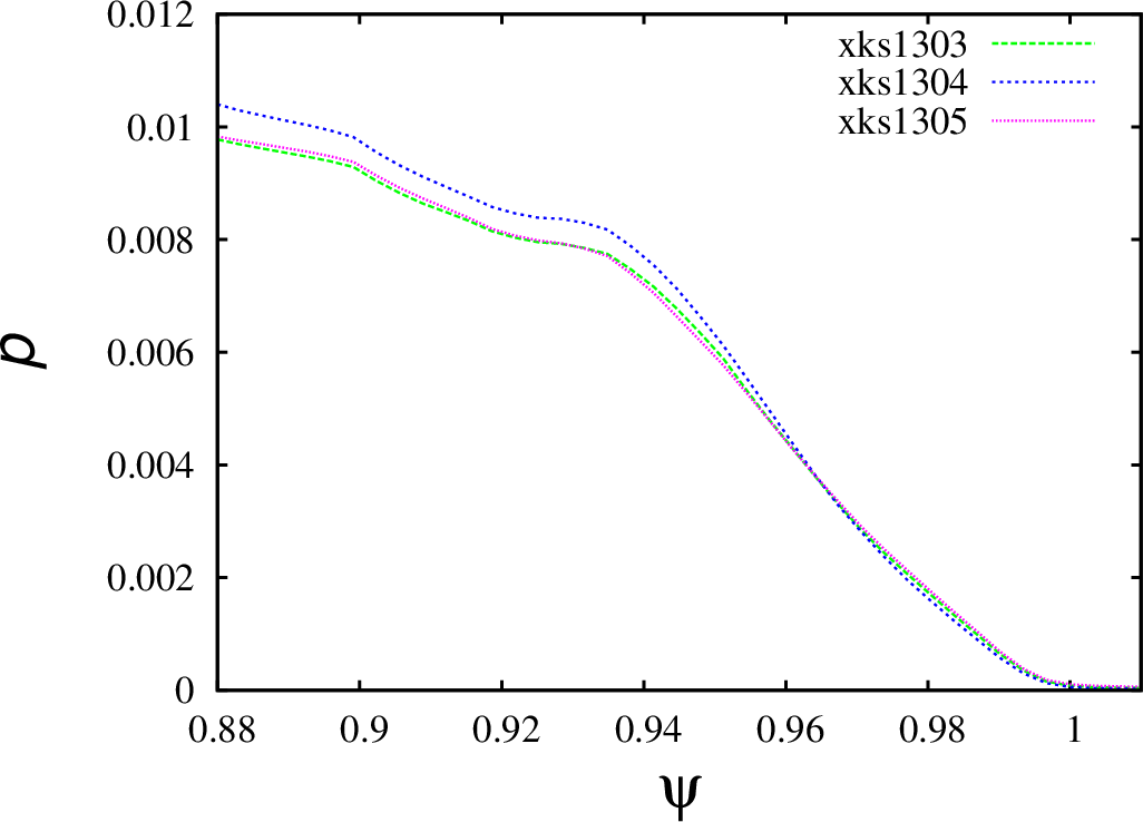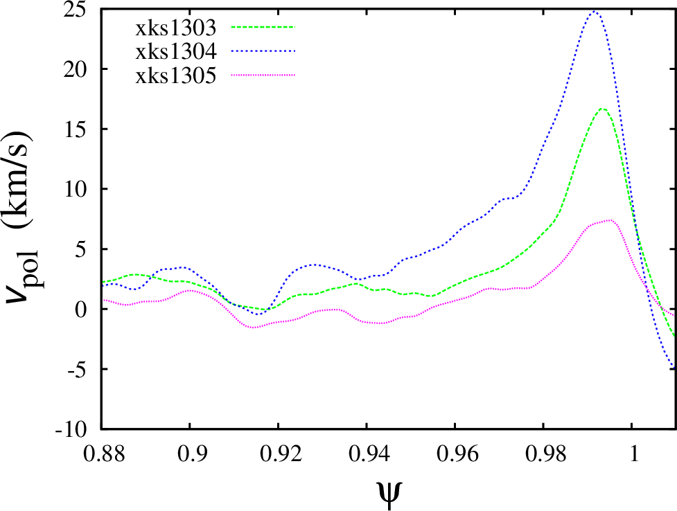The pedestal density is set to and the electron and ion temperatures are set to 500 eV. The pedestal temperature in two other XGC0 cases is varied slightly above the experimental error bars. The temperatures in the second case (xks1304) are set to 800 eV and temperatures in the third case (xks1305) are set to 300 eV. The density in these two cases are changes to keep the total plasma
pressure unchanged. The
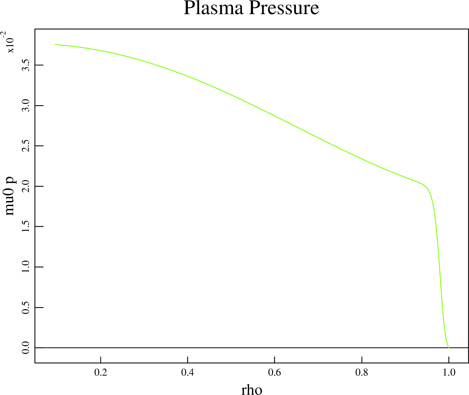
density is set to  in the case xks1304 and to  in the case xks1305. The plasma collisionality for the case xks1304 is 4.38 times smaller than the plasma collisionality in the case xks1303 and the plasma collisionality in the case xks1305 is 4.63 times larger than the plasma collisionality in the case xks1303. The plasma collisionalities for the cases xks1305 and xks1304 differ by a factor of 20. Comparing the XGC0 results for the normalized plasma pressure that are given below, one can notice that the pedestal width is reducing for the low conditionality case.
Also, the pedestal height continue to grow at larger pace for the low collisionality case. This comparison can give a range of expected pedestal widths for the initial temperatures varied within experimental error bars.

There are significant differences in the bootstrap current predictions:

The bootstrap currents differ by a factor of 2.5 for these three cases that are still within the experimental error bars.

All XGC0 profiles are smoothed to remove the MC noise. Please note that the profiles continue to evolve and XGC0 simulations for these cases will be continued until quasi-steady states are obtained.