KSTAR equilibrium reconstruction
The following steps are used for KSTAR equilibrium reconstruction:
- Generate a new inverse equilibrium using the TOQ equilibrium solver. There are certain assumptions for the plasma profiles in the process. In particular, the case s13-t00-06 uses these parameters for the plasma profiles:
 modelp=27
 nedge13=0.7
 nped13=2.6
 ncore13=4.6
 nexpin=1.1
 nexpout=1.1
 tedgeEV=70.
 tpedEV= 500
 tcoreEV=2600.0
 texpin=1.1
 texpout=2.
 widthp=.07
 xphalf=.91
- The DCON stability code is used the test the stability of resulting equilibrium
- The plasma profiles from TOQ are interpolated to the TEQ grid in Corsica. These profile include the plasma pressure and safefy factor.
- The interpolated plasma pressure and the interpolated safety factor are sent to TEQ to generated new geqdsk files that would include the vacuum field solution.
The Corsica psave and qsave variables are used.- We start with the original sav-file for this discharge:
caltrans 007328_4400.sav -probname ss-test kstar.bas - Then, we update the pressure profile and generate new inverse solution:
thetac=1e-3; epsrk=5.e-9; nht=5000; start_inv
psave( 1: 26)=[4.0652e+05,4.0636e+05,4.0589e+05,4.0510e+05,4.0400e+05,4.0259e+05,4.0085e+05,3.9876e+05,3.9636e+05,3.9354e+05,3.9038e+05,3.8681e+05,3.8290e+05,3.7861e+05,3.7397e+05,3.6897e+05,3.6364e+05,3.5798e+05,3.5201e+05,3.4573e+05,3.3917e+05,3.3235e+05,3.2528e+05,3.1798e+05,3.1047e+05,3.0278e+05]
psave( 27: 52)=[2.9493e+05,2.8693e+05,2.7881e+05,2.7061e+05,2.6233e+05,2.5400e+05,2.4565e+05,2.3729e+05,2.2897e+05,2.2067e+05,2.1246e+05,2.0432e+05,1.9630e+05,1.8841e+05,1.8065e+05,1.7307e+05,1.6566e+05,1.5845e+05,1.5144e+05,1.4466e+05,1.3810e+05,1.3179e+05,1.2572e+05,1.1991e+05,1.1436e+05,1.0907e+05]
psave( 53: 78)=[1.0405e+05,9.9302e+04,9.4818e+04,9.0599e+04,8.6643e+04,8.2945e+04,7.9499e+04,7.6298e+04,7.3334e+04,7.0596e+04,6.8068e+04,6.5736e+04,6.3577e+04,6.1565e+04,5.9667e+04,5.7842e+04,5.6037e+04,5.4183e+04,5.2207e+04,5.0025e+04,4.7558e+04,4.4737e+04,4.1586e+04,3.8103e+04,3.4179e+04,2.9900e+04]
psave( 79:101)=[2.5535e+04,2.1282e+04,1.7332e+04,1.3874e+04,1.0920e+04,8.4769e+03,6.5566e+03,5.0422e+03,3.8616e+03,2.9488e+03,2.2444e+03,1.6993e+03,1.2741e+03,9.5421e+02,7.0459e+02,5.0154e+02,3.5481e+02,2.3120e+02,1.4798e+02,8.3140e+01,3.6807e+01,8.9772e+00,3.4489e+00]
teq_inv(0,1); teq_inv(0,1)
The inverse equilibrium solver is called with the options to keep the plasma current unaltered. We run the solver two times, because the solver has a tendency to inverse the plasma current in the equilibrium solution.
- Then, the direct solution is generated using direct TEQ solver:
inv_eq=0; inv_k=0; run
- The solution is stored in a new sav-file
saveq("s13-t00-01.sav") - The q-prifiles are being updated now:
thetac=1e-3; epsrk=5.e-9; nht=5000; start_inv
qsave( 1: 26)=[1.3999e+00,1.4000e+00,1.4006e+00,1.4014e+00,1.4026e+00,1.4041e+00,1.4060e+00,1.4082e+00,1.4108e+00,1.4137e+00,1.4170e+00,1.4207e+00,1.4248e+00,1.4292e+00,1.4341e+00,1.4394e+00,1.4451e+00,1.4513e+00,1.4579e+00,1.4650e+00,1.4726e+00,1.4806e+00,1.4892e+00,1.4983e+00,1.5079e+00,1.5181e+00]
qsave( 27: 52)=[1.5289e+00,1.5403e+00,1.5524e+00,1.5650e+00,1.5784e+00,1.5924e+00,1.6072e+00,1.6227e+00,1.6390e+00,1.6560e+00,1.6740e+00,1.6927e+00,1.7124e+00,1.7331e+00,1.7546e+00,1.7773e+00,1.8009e+00,1.8257e+00,1.8515e+00,1.8786e+00,1.9070e+00,1.9366e+00,1.9675e+00,1.9998e+00,2.0336e+00,2.0689e+00]
qsave( 53: 78)=[2.1059e+00,2.1445e+00,2.1848e+00,2.2270e+00,2.2711e+00,2.3171e+00,2.3653e+00,2.4157e+00,2.4684e+00,2.5236e+00,2.5813e+00,2.6418e+00,2.7051e+00,2.7715e+00,2.8411e+00,2.9142e+00,2.9910e+00,3.0719e+00,3.1572e+00,3.2472e+00,3.3424e+00,3.4432e+00,3.5509e+00,3.6655e+00,3.7876e+00,3.9196e+00]
qsave( 79:101)=[4.0602e+00,4.2122e+00,4.3736e+00,4.5492e+00,4.7362e+00,4.9360e+00,5.1541e+00,5.3890e+00,5.6429e+00,5.9183e+00,6.2180e+00,6.5436e+00,6.8934e+00,7.2872e+00,7.7253e+00,8.1641e+00,8.6979e+00,9.1615e+00,9.8188e+00,1.0331e+01,1.0697e+01,1.0917e+01,1.0960e+01]
teq_inv(0,1); teq_inv(0,1)
- New direct solution is generated again. The solution will include the update plasma pressure and q profiles:
inv_eq=0; inv_k=0; run
saveq("s13-t00-02.sav") - Now, we need to ensure that the bootstrap current is properly included. In order to do this, we will exclude the edge current from the jparsrf and will replace it with the bootstrap current from the Sauter model:
jparsave(81:101)=jparsave(80)
real ndens=psibar; ndens=2.6e19
real prbs=psave/10./2.
real tebs=prbs/ndens/1.602e-19
real zeffbs=psave; zeffbs=1.
real pbeambs=psibar; pbeambs=0.
read jbootstrap.bas
real jbs1 = jbootstrap(prbs,ndens,tebs,tebs,zeffbs, pbeambs, 1., 1., 0.)
real jbs0 = jbs1(:,1)
real foo1=tanh((1.01-psibar)/0.05)
real foo2=(1+tanh((psibar-0.7)/0.05))/2.
jparsave=jparsave*foo1+jbs0/bsqrf*foo2
- Run a sequence of inverse and direct equilibrium solvers ensuring the the plasma current does not change:
thetac=1e-3; residj=1e-9; nht=5000; start_inv jparsave=jparsave*foo1+jbs0/bsqrf*foo2 nf; plot [jparsrf,jparsave], asrf+rsrf teq_inv(3,0); teq_inv(0,1); teq_inv(0,1) inv_eq=0; inv_k=0; run saveq("s13-t00-03.sav") - Increase the resolution in the direct equilibrium solution to 257×257 (at least):
gridup; run; saveq("s13-t00-04.sav")gridup; run; saveq("s13-t00-05.sav") - Save the new geqdsk file
weqdsk
- Note, the the resolution for the inverse solver is also important and it might be useful to increase it by changing the values of map and msrf (theta and psi dimensions in the inverse solve) and running the inverse solver.
- We start with the original sav-file for this discharge:
- The new geqdsk can be used in the MHD stability codes or with extended MHD codes for further analysis. In order to modify this equilibrium even further, one can modify the pressure profile and parallel current density profile using the last sav-file. An example below shows how to change the slope in the H-mode pedestal without changing the pedestal width:
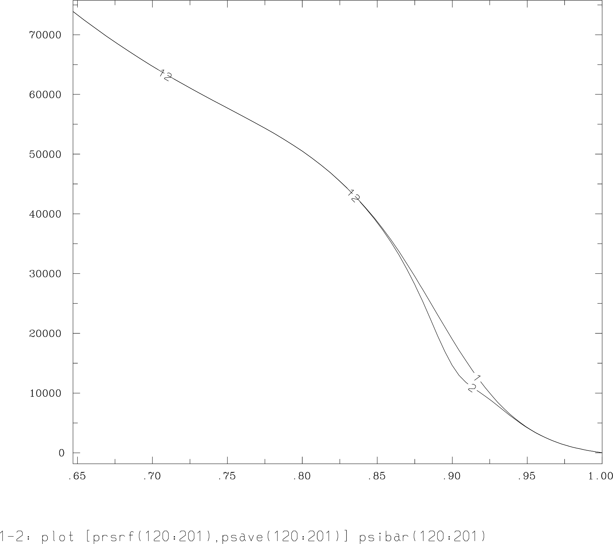
 thetac=1e-3; epsrk=5.e-9; nht=5000; start_inv
 real foo2=(1+tanh((psibar-0.90)/0.02))/2.
 real foo1=(1-tanh((psibar-0.91)/0.02))/2.
 psave=prsrf*(2-(foo1+foo2))
 teq_inv(0,1); teq_inv(0,1)
 inv_eq=0; inv_k=0; run
 saveq("s13-t01-01.sav"); weqdsk
Changes in the plasma pressure are shown below:

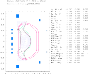
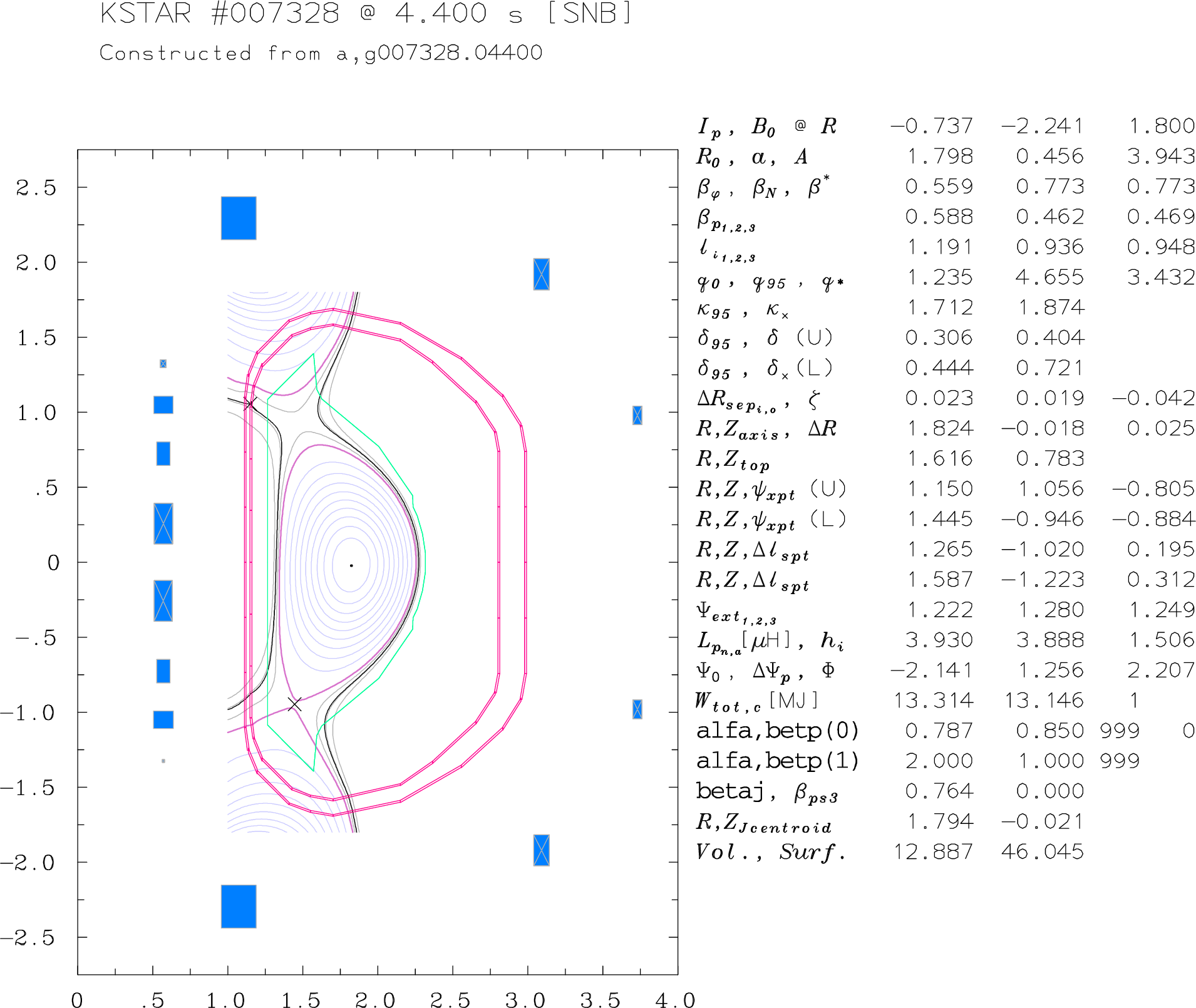
- The final layout looks as shown: